With conformal space we are concerned with angles rather than distances. We therefore don't need a complete metric which tells us what the distance between any points are, we only need to define enough to allow angles to be defined.
For example, imagine that we have a space with a set of lines meeting at certain angles and we change the scale, multiplying all distances by 'n', the distances may change but the angles at which the lines meet remain the same.
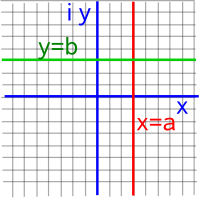
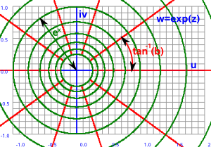
As another example of a conformal transformation, think about the exponent as a function of a complex variable, this distorts lines into circles but lines that met at 90° before the transformation (red and green lines below) still meet at 90° after. At an infinitesimal level all angles are preserved.
| z plane | w plane | |
|---|---|---|
 |
--> w=ez |
 |
Conformal space turns out to be a null space, that is all distances square to zero. In other types of space (such as Euclidean space) we might define a metric like √(Δx² + Δy² + Δz²) which defines the distance between any two points but in conformal space squaring a distance always gives zero so this would always give zero distance between any two points.
We can embed other spaces, such as Euclidean or Minkowski space, into conformal space by adding two extra dimensions to them (in a certain way that we will discuss later). Moving such spaces into conformal space can help us simplify certain problems, as might be expected in a world where angles are important, it is easier to work with rotations.
Sometimes, when modeling how solid objects move in space, we want to define a transform which can represent both rotations and transformations. This is possible in conformal space because translations can be represented as rotations with an infinite radius. Infinities can be dealt with because conformal space allows for compacification. The two extra dimensions that we add when we embed another space into conformal space are often thought of as representing the points at infinity and the points at the origin.
Conformal Space Using Clifford Algebra
Conformal Space has the advantages of projective space that we have already looked at here. These advantages include:
- Representing isometries (translations and rotations) as a single multiplication operation. This can greatly simplify the representation of objects moving in space.
- We can combine quantities to give 'meet' and 'join'.
But in addition to these, we now have the following additional benefits:
- The space is linear (we no longer need to use a shear transform).
- We can now use Clifford Algebra.
- We can now represent circles, angles etc. as quantities in our geometry.
To get these benefits there is a cost:
- We now have to embed our space in a space with two (instead of one for projective space) additional dimensions, so an 'n' dimensional space is embedded in a 'n+2' dimensional conformal space.
As usual with powerful mathematical ideas there are many possible starting points and ways to think about about the idea:
- Because the additional dimensions square to zero then the infinite series exp(x) = 1 + x1/1! + x2/2! + x3/3! ... + xr/(r)!/1! now becomes exp(x) = 1 + x so exp(iθ) = 1 + iθ.
- If rotations in Euclidean space obey spherical geometry (constant positive curvature) then the two additional dimensions obey hyperbolic geometry (constant negative curvature). By combining them in a suitable way then we can get flat space to represent transforms.
- We can think of the two additional dimensions as representing infinity and zero, that is, the infinitesimally small and the infinitely large.
- We can think of translations as being rotations with a centre at infinity.
Results
Before we delve into the theory, here is a summary of some of the useful results, so that we know where we are heading.
Conformal space adds two extra dimensions so, say 3D, Euclidean Space maps to 5D conformal space in a way that helps us represent, combine and calculate with useful quantities:
Elements
| 3D Euclidean | 5D conformal | GA Notation |
|---|---|---|
| point [x,y,z] | null vector in 5D | vector: -n0+ ½(x0²+x1²+x2²) n∞ + (x0 n1 + x1 n2 + x2 n3) |
| vector [x,y,z] | unlike point not affected by translation |
vector:
|
| Extracting plane of circle from C = P1^P2^P3 ((C^n).n).nbar= (2)p1^p2 +(-2)p1^p3 +(2)p2^p3 (p2-p1)^(p3-p1)= p1^p2 -p1^p3 +p2^p3 |
||
| two points | bivector | |
| Line through a and b | circle (defined by 3 points) special case is straight line (one of the points is ∞) |
trivector: Line : A^B^n^X = 0 = (-x2)e0^e1^e2^n∞ +(-½ + ½ x0 + ½ x1)e0^e1^n∞^n0 +(½ x2)e0^e2^n∞^n0 +(-½ x2)e1^e2^n∞^n0 |
| Circle through a, b, and c |
A^B^C^X = 0 = (-x2)e0^e1^e2^n∞ +(x2)e0^e1^e2^n0 +(-½ + ½ x0² + ½ x1² + ½ x2²)e0^e1^n∞^n0 |
|
| Hyperbolic Circle: | (A^B^e)^X = 0 = (-x2)e0^e1^e2^n∞ +(-x2)e0^e1^e2^n0 +(-½ + x0 + x1 - ½ x0² - ½ x1² - ½ x2²)e0^e1^n∞^n0 +(x2)e0^e2^n∞^n0 +(-x2)e1^e2^n∞^n0 |
|
| Plane through a, b, and d |
quadvector: A^B^n∞^D^X = 0 = (½ - ½ x0 - ½ x1 - ½x2)e0^e1^e2^n^n0 |
|
| Sphere through a, b, c, and d |
quadvector: A^B^C^D^X = 0 = (½ - ½ x0² - ½ x1² - ½ x2²)e0^e1^e2^n∞^n0 |
Where:
- X = vector in 5D conformal space
- x = vector in Euclidean space (in 3D this is x0 e1 + x1 e2 + x2 e3)
- A,B,C,D = representation of points in 5D conformal space
- a,b,c,d = representation of same points in Euclidean space
Transforms
Reflections are represented by vectors and isometries (rotation and translation) by even grades (scalar and bivector).
| 5D conformal | GA Notation |
|---|---|
| pure translation | 1 + ½(tx n∞1 + ty n∞2+ tz n∞3) |
| pure rotation | cos(θ/2) + axsin(θ/2) n23 + aysin(θ/2) n31 + azsin(θ/2) n12 |
| scaling by a scale factor of eγ | cosh(γ/2) + sinh(γ/2) n0∞ |
| reflection in plane | a1 n1 + a2 n2 |
| reflection in unit sphere | n0 - ½n∞ |
| reflection in sphere of radius eγ | |
| reflection in origin | n0∞ |
These transforms can be combined by multiplying them together, for instance, if we wish to apply a translation 't' and then apply a rotation 'r' to the result then the combined transform would be:
r*t
Transforms are applied to the elements such as points and lines by using the 'sandwich' product:
t * e * †t
where:
- t is a transform from the transform table above (translation, rotation, etc.)
- e is an element from the element table above (point, line, etc.)
- †t is the conjugate of t.
The result is of the same type as 'e' but transformed as required.
The rules for multiplying out the different basis for vectors, bivectors etc. (n1,n12 , n∞1 ...) are shown on this page (in a table at the bottom) with derivations.
Join
The outer product '^' represents the 'join' of two elements, that is the two elements and a set of points in between.
Here we will represent points by a single letter such as 'a' as follows:
a = -n0+ (x²+y²+z²) n∞ + x n1 + y n2 + z n3
Then we can combine them as follows.
| notation | GA construct | represents in homogeneous geometry |
|---|---|---|
| a | point | dual sphere (a point is a zero radius sphere) |
| a^b | outer product of two vectors | |
| a^b^c | outer product of three vectors | oriented circle |
| a^b^n∞ | outer product of three vectors (one at infinity) | oriented line |
| a^b^c^d | outer product of four vectors | oriented sphere |
| a^b^c^n∞ | outer product of four vectors (one at infinity) | oriented plane |
Meet
The inner product '•' represents the 'meet' of two elements, that is the intersection of the two elements.
Derivation for Translation between Conformal and Euclidean spaces
When we looked at projective (hemisphere and stereographic model) space we saw that it had useful properties especially for modeling and rendering 3D solid bodies using computers. However it is not practical to use clifford algebra to model projective space, if we want to do that then we need to use vectors which square to zero, to do that we need to add another dimension which squares to negative. This means that we now have two additional dimensions, added on to our euclidean space, one which squares to positive and another which squares to negative.
The constraint that we use null vectors allows us to model isometries (such as 3D solid bodies) the simplest way to do this is set the scalar value of n0 to the constant value -1. However there are advantages to compactifying the space, using the stereographic model, so that we can represent the point at infinity. This allows us to represent lines, planes, etc. as a single multivector and allows to have different transforms like reflecting in a sphere.
Null Vectors
A null vector is a vector which is not necessarily zero itself but squares to zero. Lets take a 2D euclidean space embedded in 4D conformal space:
(a n0+ b n∞ + c n1 + d n2)² = 0
where:
- n0, n∞, n1 and n2 are basis vectors described below.
- a, b, c and d are scalar values.
This will only be null if we constrain the scalar values a, b, c and d to particular values, to find these constrains we multiply out all the terms:
(a n0+ b n∞ + c n1 + d n2)*(a n0+ b n∞ + c n1 + d n2) = 0
A table showing the result of multiplying out these basis vectors is shown at the end of this page, we can see that most of the terms anti-commute (for example n1*n2= -n2*n1) and so cancel out so we are left with the scalar terms:
a*b + 2c² + 2d² = 0
So if we work in the plane a= -2 and (c,d) are the Euclidean coordinates then we b has to be:
b = 2(c² + d²)/-a
So if (u,v) is the Euclidean coordinates then our null vector is:
-n0+ 2(u²+v²) n∞ + u n1 + v n2
Stereographic Model
We can multiply the conformal vector by a scalar factor without affecting the point that it represents. This gives us the flexibility to use our null vectors in different ways.
If we set the n0 dimension to a constant value of -1 then we can represent the projective model, this is the simplest to calculate isometries , most of the examples on these pages use this model.
However we can multiply by the factor 1/(1+u²+v²), this compactifys the space using the stereographic model, so that we can represent the point at infinity. This allows us to represent lines, planes, etc. as a single multivector and allows to have different transforms like reflecting in a sphere.
| projective model | stereographic model | |||||||||||||||||||||||
|---|---|---|---|---|---|---|---|---|---|---|---|---|---|---|---|---|---|---|---|---|---|---|---|---|
| Euclidean (u,v) to conformal |
|
|
||||||||||||||||||||||
| conformal to Euclidean |
|
|
||||||||||||||||||||||
| point at origin |
|
|
||||||||||||||||||||||
| point at infinity |
|
|
We saw that the stereographic model was conformal (preserved angles) so we will start with that and add our additional dimension to it.
x² + y² + (z-1)² = 1
note: we use z-1 instead of z because the point we have chosen the origin as the point we are projecting from rather than the centre of the circle.
Now instead of constraining our vector to the unit sphere as above we constrain the vector to be a null vector:
x² + y² + (z-1)² + w² = 0
Since w squares to negative then that is equivalent to x² + y² + z² - w² = 0 if w squared to +ve.
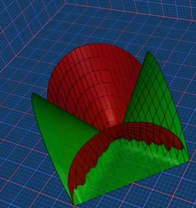
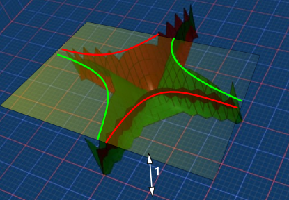
It is very difficult to visualise this in 4 dimensions so here are some special cases of this which are 3 dimensional slices through this:
If w=1 then w²= -1 which gives the unit sphere which is identical to the stereographic model:
x² + y² + (z-1)² = 1
If w=0 then w²= 0 which gives a Euclidean plane parallel to the plane at z=1 and so this only intersects at ∞ and :
x² + y² + (z-1)² = 0
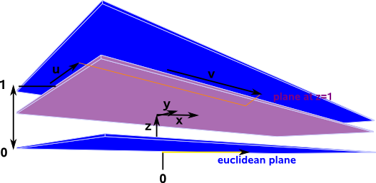
If w²= -1 we get the unit hyperbola:
x² + y² + (z-1)² = -1
Can we derive the translation between conformal and euclidean spaces by projecting using a straight line in the same way that we did for projective space.
Let us take the example of 2D euclidean space (4D conformal space).
|
= λ |
|
where:
- (x,y,z,w) = conformal coordinates
- (u,v) = euclidean coordinates
- λ = expansion factor of vector: function of (x,y,z,w)
The extra dimensions are z and w where z squares to positive and w squares to negative, that is z is real and w is imaginary.
When we apply the constraints that:
x² + y² + (z-1)² + w² = 0
and z = -1
we get:
|
= |
|
and
|
= -½ |
|
This can be simplified if we choose to rotate the z,w coordinates to get a null basis:
- n0 = (z + w)/2
- n∞ = (z - w)/2
so
- z = n0 + n∞
- w = n0 - n∞
which gives:
|
= |
|
and
|
= -½ |
|
in terms of the null vectors we have:
|
= |
|
Null Vector Basis
To create conformal space we add two extra dimensions (lets call them e1 and e2) so that e1 squares to posative and e2 squares to negative. This gives a multipication table (for these two extra dimensions alone) as follows:
a*b |
b.e | b.e1 | b.e2 | b.e12 |
| a.e | 1 | e1 | e2 | e12 |
| a.e1 | e1 | 1 | e12 | e2 |
| a.e2 | e2 | -e12 | -1 | e1 |
| a.e12 | e12 | -e2 | -e1 | 1 |
Sometimes it is useful to rotate these basis vectors by 45° to give n0 and n∞ as follows:
n0= e1 + e2
n∞= e1 - e2
This gives us a basis in terms of these null basis vectors with a multipication table as follows:
a*b |
b.n | b.n0 | b.n∞ | b.n0∞ |
| a.n | 1 | n0 |
n∞ | n0∞ |
| a.n0 | n0 | 0 | 2n0∞ | 0 |
| a.n∞ | n∞ | 4-2n0∞ | 0 | 2n∞ |
| a.n0∞ | n0∞ | 2n0 | 0 | 2n0∞ |
This table has some unusual features, the n0∞ term does not square to a scalar term.
We can see that individual products are neither commutative nor anti-commutative as we can see when we reflect the terms in the leading diagonal. However the multiplication is reasonably well behaved in that it is associative.
Points at Infinity
At infinity in Euclidean space, lets assume 2D Euclidean space, we have u=v=∞. This is not very helpful but we can apply a common multipyer without changing the point represented, so we can choose,
|
= -1/(v²+u²+1) |
|
So if we take a point at 45° at a distance of infinity so v/u=1
|
= |
|
One Dimensional Case
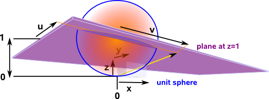
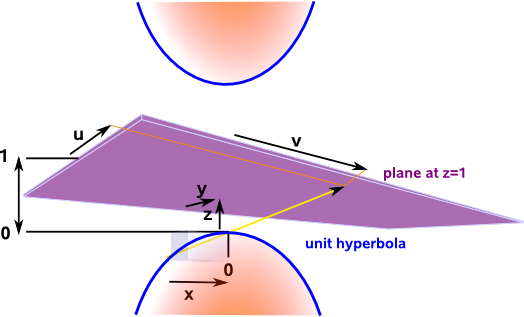
So far we have been working in 4D which is very difficult to visulaise so for now we will drop down to 1D Euclidean space which gives 3D conformal space, this may not be very useful, but it will allow us to establish the principles in a way that we can visualize.
So to represent our one dimension we will embed it in a 3 dimensional space:
Here the base (x and z dimensions) represents the two additional dimensions and the height represents another dimension in the conformal space. The green surface on the above plot represents all the points which are zero distance from the origin, that is null vectors. However this is not the usual measure of 'distance' here we are using the Minkowski metric (see Minkowski space), that is one dimension which squares to +ve and the other squares to -ve, we have also rotated these two additional dimensions by 45° so that the null at the base vectors point along the axies.
In the projective case we represented the vector where it intersected the line at y=1, in the conformal case we will represent it where the above surface intersects the plane at z=1.
Note: in this plot we have changed our usual conventions and plotted z as the up-down axis.
So because of these two constraints:
- points are represented by null vectors, zero distance from the origin, using Minkowski metric.
- z = 1
we have one degree of freedom and all the points on our one dimensional Euclidean space map to the points on the line in the diagram above.
So applying our null vector constraint to this case we have:
x² + (z-1)² + w² = 0
(x is the one dimension in euclidian space, we use no y dimension)
and the linear relationship is:
|
= λ |
|
So what are p & q?
combining
x² + (z-1)² + w² = 0
and
p=(1+u²)/2 so z = λ(1+u²)/2
which gives:
x² + (λ(1+u²)/2-1)² + w² = 0
dividing by λ²
x²/λ² + (λ(1+u²)/2-1)²/λ² + w²/λ² = 0
u + q = -(λ(1+u²)/2-1)²/λ²
in order to try to solve this lets choose:
λ = 2/(1+u²)
so
λ² = 4/(1+u²)²
which gives:
p = (1+u²)/2
q = (1-u²)/2
giving:
|
= λ |
|
Two Dimensions in 4D conformal space
This is equivalent (isomorphic to) to Dual Complex Numbers.
Higher Dimensions
We can embed euclidean space into a higher dimensional space, called conformal space, this makes transform operations involving rotations and translations easier to work with. It allows us to represent all angle preserving transformations.
When we looked at complex functions we saw that certain functions such as the inverse: (w=1/z) mapping preserve angles and we described these as conformal functions. Here we define a space where all transformations using the transform:
x = v * x * (1/v)
are conformal.
When we discussed euclidean space we said that there is no specific origin (unless we add an arbitrary coordinate system) and any point is as good as any other for zero point. Euclidean space also does not have a way to represent points at infinity.
Conformal space adds two new dimensions, one represents zero and the other represents infinity. I haven't yet got an intuitive understanding of why we need whole dimensions to represent these points.
We can now represent translations as rotations around an axis at infinity. (Its interesting to speculate if there might be a duality here to allow us to represent translations as rotations at zero?).
It is possible to represent operations, in this space, using different types of algebra, for example matrices, the most common type of algebra which we use to represent this geometry is Geometric Algebra. This is a very good match, the particular GA we use has 4 dimensions which square to +ve and one which squares to -ve, known as G4,1,0.
So we use 5 dimensions which we will denote as follows:
- e1,e2,e3 = the 3 dimensions in euclidean space
- e0 = the dimension at zero
- e∞ = the dimension at infinity.
The way that we use this algebra to represent translations and rotations is described on this page.