Types of Clifford Algebra
This section introduces whole classes of algebras that can be defined in multiple dimensions. We will call an element in this algebra a multivector. These algebras have different types of multiplication that can be applied to a given multivector.
These classes of algebras are summarised in the following table.
| Type | Metric | Description |
|---|---|---|
| Grassmann Algebra |
This introduces a new vector multiplication (exterior product) denoted by '/\' which anticommutes and quantities square to zero. This creates a graded structure from the bases to create higher order bases. So in addition to the dimension of the underlying vector algebra the algebra also has a 'rank' which is the maximum size of these higher order bases. This Grassmann algebra provides a framework for Clifford algebra. | |
| Orthogonal inner and Clifford products. |
 |
In addition to the exterior product from Grassmann product we add a inner product (which may be denoted '•' or '\/' to denote a duality with the exterior product) where unit quantities square to +1 or -1. The Clifford product can then be defined from a combination of exterior and inner products. There are also other flavors of the inner product such as the left '|_' or right '_|' contraction products. This form of Clifford product contains algebras such as complex numbers and quaternions. This can be applied to rotation in 'n' dimensional Euclidean space or in spaces such as Minkowski where some dimensions square to -ve. |
| Quadratic Form |
 |
In addition to allowing dimensions to square to +ve or -ve we now allow these dimensions to be rotated. For example at some point between squaring to +ve and -ve there will be a case where the dimension squares to zero. This is is useful geometrically because it allows us to combine rotations and translations and into a single transform using this form of the Clifford multiplication. There are a number of spaces such as projective and conformal space which allow us to do this. This is the main application of Clifford algebra on this site. |
| Bilinear Form |
 |
This makes the inner product even more general and so it is not constrained to be a quadratic form but can be any bilinear form. Analysis of this case can be found in papers by Rafal Ablamowicz and Bertfried Fauser. |
Geometric Algebra (GA)
We will start with Geometric Algebra (GA).
Its always difficult to learn a new type of algebra, at first it feels like learning a lot of arbitrary rules and its only when this hard work is done that the relationship to other algebras becomes apparent. I think the effort in learning Geometric Algebra (GA) could be worthwhile both, because of the way that it generalises both vector algebra and quaternions, also in terms of the subject matter of this site because of the potential to provide more powerful tools for working out solid body mechanics problems.
There are a number of different ways to think about this algebra, different people might react differently to the ways to describe Geometric Algebra (GA), an approach that may not help one person may just help the whole thing 'click' with another person. I have therefore included pages to describe the following approaches:
- A more theoretical introduction to GA
- As a modification and extension of vector dot and cross products.
- Geometrical interpretations.
- Defining multiplication rules using tables.
- Other papers.
Geometric Algebra is as an extension of Vector Algebra
When we discussed vector algebra we had two types of multiplication:
- A dot product takes two vectors and produces a scalar.
- A cross product takes two vectors and produces a bivector.
Having two types of multiplication which give outputs that are not vectors is not altogether satisfactory. these operations are useful in that they have lots of practical applications. However, in mathematical terms, it would be better if we had a vector algebra that was 'closed' that is the outputs of the operations have the same form as the inputs.
This is not possible for vector algebra but it is possible if our elements are a superset of scalars, vectors, bivectors and higher order components. We can then define a general multiplication which is a combination of cross and dot multiplication.
As a first stage imagine a 3D vector as a linear sum of base vectors e1, e2 and e3.
v = a1 e1 + a2 e2 + a3 e3
where:
- v = vector being defined.
- e1, e2 and e3 are independent, unit length base vectors.
- a1, a2 and a3 are scalar values which give the elements of the vector..
Now we could extend this to made a new type of quantity
m = a0 + a1 e1 + a2 e2 + a3 e3
where:
- m = extended vector (which will eventually become a multivector)
This means that the dot, cross and scalar products mentioned above now have both inputs and output as members of this new type of extended vector. However the operations are still not general in that these operations only apply to a subset of the multivectors.
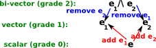
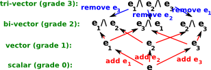
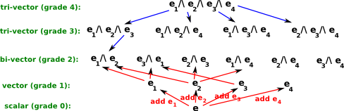
We will now define a new type of product, which is more general, it is called the outer product and it is denoted by '/\'. This type of multiplication has similar properties to the vector cross product but it applies to any number of dimensions. When we use it to multiply a vector, say e1, by a different vector, say e2, then this generates a new type e1/\e2 which can't be further simplified. If we then multiply by another vector, say e3, then this will produce yet a further new type e1/\e2/\e3 and so on.
At first sight it would seem that this will potentially produce an infinite number of types, but that is not so, an algebra based on vectors of dimension 'n' will generate 2n scalar elements in a multivector (including the scalar and the original vector). The reason that the number of types does not keep growing is that the above rules only apply if the vectors are different, if we multiply the vector by itself the result is zero so: e1/\e1 = 0. This type of algebra, where a quantity is not zero, but squaring it makes it zero is known as a grassmann algebra. If we have an element, say e1/\e2, and we multiply it by an element that is already included in the first, say e2, then these two e2s will cancel out and we will be left with e1. If the duplicate terms are not adjacent then there may be a sign change (+ to - or - to +) because the '/\' operator is antisymmetric.
So the quantities in this algebra consist of 2n scalar values (some of which may be zero and therefore not written) .In the same way that vector algebra may be different depending on the dimension of the vectors, geometric algebra depends on the dimension of the vectors contained in it. The elements (equivalents to numbers - i.e. the object we are manipulating) in geometric algebra are known as multivectors (or alternatively monads). in other words:
- in real algebra we work with numbers.
- in vector algebra we work with vectors.
- in complex algebra we work with complex numbers.
- in matrix algebra we work with matrices.
- in geometric algebra we work with multivectors (some books use the term monads).
These multivectors are made up of blades and each blade has a grade as well as a dimension.
- Grade 0 is a scalar number (which has dimension 1) ,
- Grade 1 is a vector (whose dimension determines the number and dimension of the remaining grades) ,
- Grade 2 is a bivector (whose dimension depends on the vector) ,
- And so on for tri-vectors...
When blades of different grade are added the result cannot be simplified further and the multivector is just the sum of these with the '+' sign left in. This is the same principle as the notation for complex numbers or quaternions which might be denoted by say the number 2+i3 which cannot be further simplified.
Hopefully this will become clearer later when we derive multivectors from different dimension vectors.
Perhaps we can start here with three dimensional vector algebra, the rules are changed slightly, in a way that generalises the result.
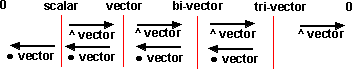
We replace the dot, cross and scalar products of vector algebra with the following operations for geometric algebra:
- Inner product (•) replaces and extends dot product and for vectors is defined in the same way.
- Outer product (/\) replaces and extends cross product.
- Geometric product is the main type of multiplication used in geometric algebra, this type of multiplication is denoted by * and is implied when we put the multiplicands next to each other without using a multiplication symbol.
The small change in the rules is that the outer product of two vectors results in a new entity called a bivector, there may also be tri-vectors and so on. depending on the dimension of the vectors. Multiplying by a vector using the outer product increases the grade of the result by 1, multiplying by a vector using the inner product decreases the grade of the result by 1, so these operations have a nice symmetry.
The outer product is denoted by /\ When two independent base vectors are outer multiplied, for instance e1/\ e2, we cant further simplify the result so we just leave the result as: e1/\ e2.
Note: in Hestenes the base vectors are denoted by sigma (σ1,σ2, etc.) but these are a bit more difficult to write in web pages and programming languages so I am using e1, e2, etc. to denote base vectors.
In the general case a multivector may contain all possible combinations (not permutations) of the base vectors. In other words we only need to include e1/\ e2 or e2/\ e1 but not both. This is because the /\ operator anti-commutes (e1/\ e2 = - e2/\ e1) so if we choose e1/\ e2 as the bivector then if we have any e2/\ e1 terms we can use minus the e1/\ e2 term instead . Also we don't have any terms occurring more than once. If a term such as e1/\ e1 occurs then this can be replaced by a scalar value, this is because e1/\ e1 = 1 or -1 depending on how it is defined. By the anti-commute rule then e1/\ e1 = - e1/\ e1 which would only be true if e1/\ e1=0 but this can give the desired result as explained here.
Geometric Product
The outer product gives zero if there are two, or more, of any particular base, for instance,
(e2/\e1)/\e1=0
The geometric product does not produce zero unless the operands are zero, for instance,
(e2/\e1)*e1=e2
So this geometric product has properties much more like other algebras and it can generate algebras which are equivalent to complex numbers, quaternions, etc.
When we are working with vectors the geometric product is a sum of the inner and outer products:
e1*e2 = e1/\e2 + e1•e2
Does this work with general multivectors x and y:
x*y = x/\y + x•y
This does not necessarily work for all multivectors, although it seems to work for a bivector times a vector:
(e2/\e1)*e2 = (e2/\e1)/\e2 + (e2/\e1)•e2 = 0-e1= -e1
So this seems to work provided that (e1/\e2).e2 = e1/\(e2.e2) ? It would be good to define when this holds, obviously it depends what type of inner product we use. I would like to understand more about the rules for inner and outer products.
So with the geometric product, if the same base occurs on both sides of the product it cancels out to '1' so:
e1*e1=1
but there may be a sign change, the rules for calculating the sign are explained on this page.
Choice of bases
If we want to have a standardised representation of multivectors then we need to choose:
- factor ordering - this affects the sign for example: e13= -e31
- element ordering - if we want to represent a multivector as a list we have to choose the order that the elements are put in the list.
Possible options for factor ordering are:
- dually - such that for grade 3:
I2e1* = e23
I2e2* = e31
I2e3* = e12 - index sequentially e12,e13,e23
where:
- I = pseudoscalar (e123 in 3D)
- a* is the dual of a
Textbooks (such as Hestenes) choose pseudoscalar 'I' such that it has the orientation specified by a right-handed set of vectors in 3D. The dual function alone does not define the factor ordering, we can still swap factors and invert the sign. We need to use the determinant as explained here.
Possible options for element ordering are:
- grade-ordered {1,e1,e2,e3,e23,e31,e12,e123}
- bitwise-ordered {1,e1,e2,e12,e3,e13,e23,e123}
The advantage of bitwise ordering is that a grade 3 multivector is just an extension of a grade 2 multivector and so on.