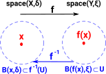
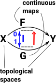
Continuity Between Metric Spaces
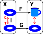
Even if we are mostly interested in continuity between non-metric spaces I think it helps intuition if we look at metric spaces first. The diagram shows a function from X with a metric δ to Y with a metric ξ. We have an open set which is a ball around x and an open set which is a ball around f(x). For continuity, as the ball around x gets smaller we want the ball around f(x) to get smaller. |
 |
| To visualise this as a function better lets draw these balls in two dimensions only: | 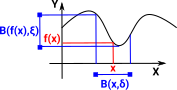 |
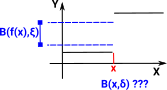
| As an example of a function that is not continuous lets take a function that has value 1 when x<3 and has value 4 when x<=3. |  |
Here we can see that there is a smaller ball (open set) in Y but it doesn't have a corresponding ball (open set) in X. So we can start to see that there is a requirement, for continuity, that open sets in Y map through f-1 to open sets in X. |
 |
Continuity between Finite Spaces
In addition to the examples above we can also have continuity between non-metric and finite spaces.
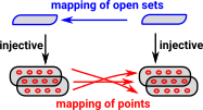
Here we are mapping elements of topological spaces (open sets).
Continuous maps conserve topological properties. The following examples are intended to show how continuous maps preserve 'connectedness'.
 |
In this diagram we have a map which takes two unconnected open sets ('A' and 'B') to one open set 'X'. This is like pulling together a tear between 'A' and 'B'. This is not a continuous map because the open set 'X' does not have a pre-image. |
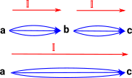
In this diagram we have a map which takes two connected (overlapping) open sets ('A' and 'B') and their union to one open set 'X'. This conserves the connected property. This is now a continuous map because the open set 'X' does now have a pre-image AUB. |
 |
 |
In this diagram we have a map which takes one open set 'X' to two unconnected open sets ('A' and 'B') to. This is like making a tear between 'A' and 'B'. This is not a continuous map because the open set 'B' does not have a pre-image. |
In this diagram we have a map which takes one open set 'X' to two connected (overlapping) open sets ('A' and 'B'). This is a continuous map because all the open sets in the codomain have a pre-image. |
 |
 |
In this diagram we have a map which takes two unconnected open sets ('A' and 'B') to two other unconnected open sets ('X' and 'Y'). This conserves the connected (or in this case unconnected) property. This is a continuous map because all the open sets in the codomain have a pre-image. |
The same principles apply for higher dimensional holes. Here there is a hole inbetween'A','B' and 'C'. That is there is no 'A ' U ' B ' U ' C' so 'X' does not have a pre-image. |
 |
 |
If 'A', 'B' and 'C' are extended then 'A ' U ' B ' U ' C' exists so 'X' does have a pre-image and the map is continuous. |
| Another, more complicated, example is that the continuous map could merge f'A' and 'B' together (but not 'C' ). This would givea valid continuous map with two intersections both ('X' |
 |
More about this subject on page here.
Continuous Maps
A function is continuous if it doesn't jump, that is, when two inputs of the function get close to each other then the corresponding outputs of the function get close to each other.
Here we discuss the most general form of continuous map which also applies to non-metric topological spaces.
A continuous mapping implies a limited kind of reversibility, at least locally.
Definition 1
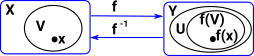
Here is one definition of continuity, based on open sets:
| Let X and Y be topological spaces. A function f : X->Y is continuous if f-1(V) is open for every open set V in Y. | 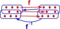 |
Definition 2
Another definition of continuity, based on neighbourhoods, is equivalent to the above definition.
| Let X and Y be topological spaces. A function f : X->Y is continuous if for every x |
 |
More detail about continuity on page here.
Continuous Surjective Maps
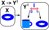
Here is an extreme case of a Surjective Map which maps to a single point. This seems to meet the requirements as there is an open set round the whole preimage. We can think of surjections which meet these requirements as 'nice surjections'. See fibrations |
Continuous Injective Maps
Here is an extreme case of a Injective Map which maps from a single point. In this case all the open sets in the codomain need to map back to a single open set in the domain. This meets the requirements so it is a 'nice injection'. See cofibrations |
Continuity as Pullback
This diagram shows a set of points being mapped to another set of points (in red). For that map to be continuous the pre-image of every open set must be an open set (shown as blue map in the reverse direction). |
 |
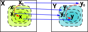
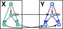
Continuity and Limits
In the continuity between metric spaces examples at the top of this page we reduce the ball in the codomain and the ball in the domain must also reduce as the map is continuous.
The limit is when the ball in the codomain and the domain both reduce to a single point.
This idea of a limit generalises to continuous maps between non-metric topological spaces.
See page here about categorical limits.
Continuous Maps Preserve Limits
 |
Topology PerspectiveLet X and Y be topological spaces. A function f : X->Y is continuous if for every x |
Category Theory PerspectiveThe category Top has topological spaces as objects and continuous maps as morphisms. The isomorphisms in this category correspond to homeomorphisms in topology. Top preserves limits and co-limits. Simplicial sets are co-limits of Top. Top is a category but it does not have exponential objects for all spaces and so it does not have some nice properties: it is not cartesian closed or a topos. If these properties are required then there may be variations of Top for the spaces required that have these properties. For example, nice topological spaces such as compactly generated topological spaces. Or see homotopy category at ncatlib. See page here about categorical limits. |
 |
Continuity of Maps between Lattice Structures
| So far we have drawn diagrams with intersections and unions (Venn diagrams) but we could also draw these in terms of logic. | 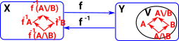 |
Examples
| In this diagram the points stay within their open sets. This is a continuous map, the pre-image of every open set is an open set. The intersections and unions of open sets play nicely together. | 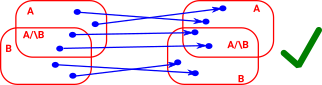 |
| This next example is not a continuous map because the preimage of A is not an open set because it includes A and A/\B but not B. We could think of this as a tear. | 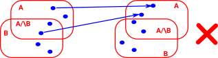 |
| Again this example is not a continuous map because the preimage of A is not an open set. | 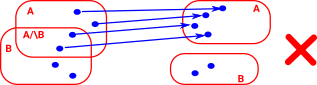 |
| In this example the whole space is shrunk to a point. This is a valid continuous map because the preimage A\/B is an open set. | 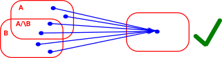 |
Homotopy
 |
If we have two topological spaces X & Y with two continuous maps between them F & G then a homotopy is a continuous map between F & G. In order to see how this is related to the map between the cup and torus I have drawn a map from a third shape (in this case another torus). So as F continuously maps the G then the cup maps to the torus. |
We can move the continuous map forward from the functions to the domain so the functions are homotopic if:
where:
We can think of this as 'filling in' the gap between F and G so that we can take any path through it. |
 |
 |
Or we can draw it in the codomain (currying) so that each element in X maps to I->Y. |
More about homotopy on page here.
 |
Maps F & G are homotopic if:
where:
We can think of this as 'filling in' the gap between F and G so that we can take any path through it. There is a good video about this on a site here. |
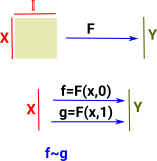
A homotopy is a function between functions with certain properties.
Let X and Y be topological spaces and f,g : X->Y be two continuous maps. Then f is said to be homotopic to g (written f~g) if there exists a map F : X× where:
|
 |
Fibrations and Continuous Maps
Some continuous maps between spaces have a 1:1 mapping between points, these continuous maps are known as homeomorphisms. It is also possible to have a continuous map from a line to a point, or vise versa, that is what we are discussing here.
 |
There is a continuous map from a line to a point. In the same way that in sets, attempting to reverse a surjective map leads to fibre bundles, with continous maps we get fibrations. |
 |
This continuous map is reversible so we have a continuous map from a point to a line. |
| So, for example, two circles that touch at a point can be continuously deformed into a circle with a line through the middle. | 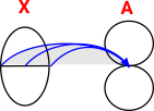 |
Or we can expand all the points on, say a circle, to get a band. This is like a product of a circle and a line. |
 |
For more information see:
Transport
| from here | transport : Path U A B -> A -> B |
That is, if we have a path from A to B and A, then B.
Composition of Paths
We want to compose these two paths:
|
 |
from here 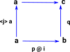 |
compPath (A : U) (a b c : A) (p : Path A a b) (q : Path A b c) : Path A a c =
comp (<_> A) (p @ i)
[ (i = 0) ->
Where 'comp' is a keyword with the following parameters:
|
