Homology

Homology Groups - Use as Invariants

As introduced on page here: In two dimensions it is relatively easy to determine if two spaces are topologically equivalent (homeomorphic). We can check if they:

are connected in the same way.
have the same number of holes.

However, when we scale up to higher dimensions this does not work and it can become impossible to determine homeomorphism. There are methods which will, at least, allow us to prove more formally when topological objects are not homeomorphic.

These methods use 'invariants': properties of topological objects which do not change when going through a homeomorphism. Here we look at invariants which arise from homology. The page here discusses different invariants which arise from homotopy, which can be harder to work with but may be more selective.

Computing Homology Groups

When we looked at the delta complex we got a chain of 'face maps' between each dimension and the next lower one.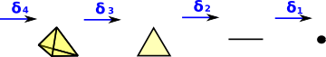

In homology we treat this as a chain of Abelian groups.

The boundary of a simplex is not a simplex, but a chain with coefficients 1 or −1. So chains are the closure of simplices under the boundary operator

Here is an outline of an algorithm to compute the homology group from a simplicial complex:

Start with Simplicial Complex

Start with a simplicial complex, in this case 3 vertices with edges forming a circle.

Compute Geometric Realisation

Convert vertices, edges and higher order faces to (basis) vectors.

So each of the vertices is a vector in its own dimension. They form a set of basis vectors.

More about geometric realisation on page here.

All the higher order faces are also represented as a set of (basis) vectors.

Compute Chain Complex

Relate the vertex vectors, edge vectors ... by matrices.

More about chain complex on page here.

Compute Smith Normal Form

Convert these matrices to Smith normal form as described below.

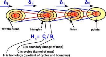
Compute Homology Groups

Homology is cycles modulo boundary.

The homology at each step in the chain measures the connectivity of the space. The outer yellow area shows new elements that have been added in at that layer, inside that are elements that have been inherited from higher layers.

Torsion

The chain complex uses matrices which must be defined over a type which has addition and multiplication. So it can be defined over a Field or a Ring.

If it is defined over a ring of integers (Z) then we have types like Z/2, for example,

C_k=ZZ/2

Fractional integer types such as Z/2 are required because the terms in a ring cant be fractional. If the matrices are defined over a field then these torsion types are not required.

Möbius Band - Example of Torsion

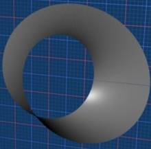
If Z represents all the ways a path can wind around a hole then Z/2 might occur in a shape such as a Möbius band where a path has to go round twice to get back to where it started.

More about computing Möbius band on page here.
More about torsion on page here.

Here is a simplicial complex for the Möbius band.

The two blue arrows are glued together in the direction shown to give a twist in the band.

I've divided the square into 2 triangles to make it into a simplicial complex although that's not very relevant here.

In this diagram I have taken a second copy of the Möbius band, the second one is flipped vertically, so that they fit together

The red arrows indicate a path twice around the band so that it gets back to where it started and forms a cycle.

As we go around this cyclic path we can go in the direction of the oriented edges (indicated by black arrows) and also in the opposite direction.

At each vertex we can add up the edges where an incoming (black) arrow is +1 and an outgoing arrow is -1.

So if the path is in the same direction of the edges then the incoming and outgoing edges cancel out and each vertex has the value 0.

Where two edges meet at the vertex we get the value +2. Where two edges exit the vertex we get the value -2.

So the value of the path at each vertex is always an even number. This is because we are using integers (Z). If we could use fractional values (Field) in the matrix we could arrange for the vertex values along the path to be -1,0 or +1.

Smith Normal Form

The following operations on a matrix are reversible:

Swapping rows.
Adding a multiple of one row to another.
Multiplying a row by an integer.

We can do each of these operations, or combinations of them, by multiplying with a square matrix. Then we can get back to the original matrix by multiplying by the inverse square matrix. We can do the same operations on columns by post-multiplying by the square matrix instead of pre-multiplying.

Doing these operations allows us to get to a diagonal matrix from any arbitrary matrix.

Idea for this diagram comes from this website.

The above applies to a matrix over a field or. more specifically over a principle idea domain (PID)

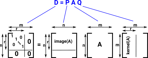
If we work with an integer matrix then, instead of the diagonal of D containing 1's and 0's it now contains invariant factors of A:

b₁ ≤ b₂ ≤...≤ b_r

if b_i ≠1 this is torsion Z/a

b₁	0	0		0
0	b₂	0	…
0	0	b₃

0				0

We use the Smith normal form by calculating from the face maps in linear algebra (matrix) form.

Once in this form we interpret it as follows:

H = Z _b1Z _b2Z _b3…

Homology Groups in FriCAS

If A is matrix for D_k+1 and B is matrix for D_k, so that B*A = 0, then torsion part of homology can be read directly from the Smith form of A: rows of leftEqMat give you generators and diagonal entries give order. If diagonal entry is 1, then coresponding cyclic group is trivial and generator is not needed at all. In the case above we get:

[1 0 0] of order 2
[- 1 3 2] of order 6
[3 - 4 - 3] of order 12

as generators of torsion part. Note that torsion part depends only on A, as long as B*A = 0 it does not depend on B. Since A is of full rank in this case free part of homology group is trivial, so the generators above give full description of homology. In general free part of homology may be computed over rational. We can use the following trick: let W be kernel of B treated as matrix over rationals and let V be ortogonal complement of image of A (again over rationals). Now W/Im(A) isomorphic to W \cap V. V is kernel of transpose(A), so to compute W \cap V it is enough to compute kernel of C := horizConcat(B, transpose(A)). You can use completeSmith to get integer basis of this kernel.

From Waldek Hebisch post here:

https://groups.google.com/g/fricas-devel/c/mLOdQ-fwbO0

Homology - Comparison with Homotopy

In homology we don't just use n-spheres but every closed oriented n-dimensional sub-manifold.

It also uses a different definition of equivalence classes where composition of loops commutes. This results in Abelian groups.

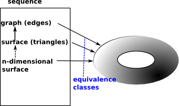So we don't need to fix the basepoint.

If you have not already done so I suggest you read the page about Simplicial Complexes first and also general introduction here.

Homology is an equivalence between cycles in a topological space. On this page we look at code to test this equivalence.

Calculating Homology from Simplexes

Matrix Form of Face Maps

We can represent these face maps by matrix representations, this allows us to relate to linear algebra methods.

We can then generate the homology by putting them in Smith normal form (which is already implemented in Axiom/FriCAS).

Example for Tetrahedron

Here are the face maps as discussed on the delta complex page here.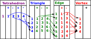

We can convert this to a matrices as follows:

Face map

Matrix

δ₃ = tetrahedron to triangles

from 1 tetrahedron

to triangle 1 to 4

-1

δ₂ = triangles to edges

from triangle 1 to 4

to edge 1 to 6

1	1	0	0
-1	0	1	0
0	-1	-1	0
1	0	0	1
0	1	0	-1
0	0	-1	1

δ₁ = edges to vertices

from edges 1 to 6

to vertex 1 to 4

1	1	1	0	0	0
-1	0	0	1	1	0
0	-1	0	-1	0	1
0	0	-1	0	-1	-1

For these face maps to be valid chain they must be:

Composible - number of columns in δ₁must equal number of rows in δ₂.
Product is zero - δ₁* δ₂ = 0

Chains

In the case of edges we can chain them together.

A cycle is any combination of edges where at least one decomposition into cycles exists.

Graph Example

H₁(X) = Z^e-v+1

Orientation and Notation

Getting a consistent orientation naming/numbering is very important. We therefore need to take some time to define it precisely

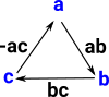
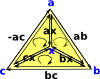
Lets start with a 2-dimensional face, that is, a triangle:

Here it is denoted [a,b,c].

It is oriented, that is, as it is drawn here it has a clockwise orientation. An anti-clockwise triangle such as [a,c,b] can be thought of as an inverse.

Here we will denote the edges as bc, ca and ab but it is easier if the nodes are alphabetically ordered, so instead we denote the edges:

bc, -ac and ab

So now each edge is designated in alphabetical order and the middle edge is negative.

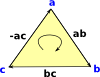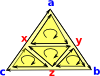
We can subdivide the triangle by adding another node 'x' as shown in the diagram:

This allows us to create 3 triangles. Provided that each of these has a clockwise orientation then,

The external edges will have the same direction as the original triangle.

The internal edges will each have two edges in opposite directions, so we can think of them as canceling out, leaving us with the original triangle. So,

[a,b,c] = [b,c] - [a,c] + [a,b]

Designating the triangles in terms of their edges we have:

[bc, -ac , ab ] =
[bc, -xc , xb ] - [ac, -xc , xa ] + [ab, -xb , xa ]

In theory we could divide each triangle up into 4, by splitting each edge, like this:

However we don't tend to use this method because:

Dividing external edges would force us to do the same to adjoining triangles which would force us to subdivide the whole surface.
This method does not necessarily work for dividing higher dimensional faces.

Calculated Examples

The only way I could think of to try to validate my FriCAS code is to compare it with the same calculations in SAGE. The sage examples are taken from my SAGE worksheet here. Of course, these are simple examples, so even if they agree it does not necessarily mean my code is correct.

Disc (filled in circle) an 2-sphere examples

gives H0=Z, H1= 0, H2 = 0

SAGE	FriCAS
S2 = simplicial_complexes.Sphere(2) S2.homology() {0: 0, 1: 0, 2: Z} S3 = simplicial_complexes.Sphere(3) S3.homology() {0: 0, 1: 0, 2: 0, 3: Z}	(1) -> b1 := sphereSolid(2)$SimplicialComplexFactory (1) (1,2,3) Type: FiniteSimplicialComplex(VertexSetAbstract) (2) -> homology(b1) (2) [Z,0,0] Type: List(Homology) (3) -> b2 := sphereSolid(3)$SimplicialComplexFactory (3) (1,2,3,4) Type: FiniteSimplicialComplex(VertexSetAbstract) (4) -> homology(b2) (4) [Z,0,0,0] Type: List(Homology)

SAGE

FriCAS

S2 = simplicial_complexes.Sphere(2)
S2.homology()
{0: 0, 1: 0, 2: Z}


S3 = simplicial_complexes.Sphere(3)
S3.homology()
{0: 0, 1: 0, 2: 0, 3: Z}

(1) -> b1 := sphereSolid(2)$SimplicialComplexFactory

   (1)
        (1,2,3)
         Type: FiniteSimplicialComplex(VertexSetAbstract)
(2) -> homology(b1)

   (2)  [Z,0,0]
                                     Type: List(Homology)
(3) -> b2 := sphereSolid(3)$SimplicialComplexFactory

   (3)
        (1,2,3,4)
         Type: FiniteSimplicialComplex(VertexSetAbstract)
(4) -> homology(b2)

   (4)  [Z,0,0,0]
                                     Type: List(Homology)

Sphere and Disc Surface (Boundary) Example

youtube example

gives H0=Z, H1= Z, Hn = 0 {n>1}

SAGE	FriCAS
BS2 = SimplicialComplex([[0,1], [1,2], [0,2]]) BS2.homology() {0: 0, 1: Z}	(5) -> b3 := sphereSurface(2)$SimplicialComplexFactory (5) (1,2) -(1,3) (2,3) Type: FiniteSimplicialComplex(VertexSetAbstract) (6) -> homology(b3) (6) [Z,Z] Type: List(Homology) (7) -> b4 := sphereSurface(3)$SimplicialComplexFactory (7) (1,2,3) -(1,2,4) (1,3,4) -(2,3,4) Type: FiniteSimplicialComplex(VertexSetAbstract) (8) -> homology(b4) (8) [Z,0,Z] Type: List(Homology)

SAGE

FriCAS

BS2 = SimplicialComplex([[0,1], [1,2], [0,2]])
BS2.homology()
{0: 0, 1: Z}

(5) -> b3 := sphereSurface(2)$SimplicialComplexFactory

   (5)
        (1,2)
        -(1,3)
        (2,3)
         Type: FiniteSimplicialComplex(VertexSetAbstract)
(6) -> homology(b3)

   (6)  [Z,Z]
                                     Type: List(Homology)
(7) -> b4 := sphereSurface(3)$SimplicialComplexFactory

   (7)
        (1,2,3)
        -(1,2,4)
        (1,3,4)
        -(2,3,4)
         Type: FiniteSimplicialComplex(VertexSetAbstract)
(8) -> homology(b4)

   (8)  [Z,0,Z]
                                     Type: List(Homology)

Torus example

SAGE	FriCAS
RP3 = simplicial_complexes.Torus() RP3.homology() {0: 0, 1: Z x Z, 2: Z}	(9) -> b5 := torusSurface()$SimplicialComplexFactory (9) (1,2,3) (2,3,5) (2,4,5) (2,4,7) (1,2,6) (2,6,7) (3,4,6) (3,5,6) (3,4,7) (1,3,7) (1,4,5) (1,4,6) (5,6,7) (1,5,7) Type: FiniteSimplicialComplex(VertexSetAbstract) (10) -> homology(b5) (10) [Z,Z*2,Z] Type: List(Homology)

SAGE

FriCAS

RP3 = simplicial_complexes.Torus()
RP3.homology()
{0: 0, 1: Z x Z, 2: Z}

(9) -> b5 := torusSurface()$SimplicialComplexFactory

   (9)
        (1,2,3)
        (2,3,5)
        (2,4,5)
        (2,4,7)
        (1,2,6)
        (2,6,7)
        (3,4,6)
        (3,5,6)
        (3,4,7)
        (1,3,7)
        (1,4,5)
        (1,4,6)
        (5,6,7)
        (1,5,7)
          Type: FiniteSimplicialComplex(VertexSetAbstract)
(10) -> homology(b5)

   (10)  [Z,Z*2,Z]
                                     Type: List(Homology)

Real projective space example

SAGE	FriCAS
RP4 = simplicial_complexes. RealProjectiveSpace(2) RP4.homology() {0: 0, 1: C2, 2: 0}	(11) -> b6 := projectivePlane()$SimplicialComplexFactory (11) (1,2,3) (1,3,4) (1,2,6) (1,5,6) (1,4,5) (2,3,5) (2,4,5) (2,4,6) (3,4,6) (3,5,6) Type: FiniteSimplicialComplex(VertexSetAbstract) (12) -> homology(b6) (12) [Z,C2,0] Type: List(Homology)

SAGE

FriCAS


RP4 = simplicial_complexes.
                           RealProjectiveSpace(2)
RP4.homology()

{0: 0, 1: C2, 2: 0}

(11) -> b6 := projectivePlane()$SimplicialComplexFactory

   (11)
         (1,2,3)
         (1,3,4)
         (1,2,6)
         (1,5,6)
         (1,4,5)
         (2,3,5)
         (2,4,5)
         (2,4,6)
         (3,4,6)
         (3,5,6)
          Type: FiniteSimplicialComplex(VertexSetAbstract)
(12) -> homology(b6)

   (12)  [Z,C2,0]
                                      Type: List(Homology)

Klein bottle example

SAGE	FriCAS
RP5 = simplicial_complexes. KleinBottle() RP5.homology() {0: 0, 1: Z x C2, 2: 0}	(13) -> b7 := kleinBottle()$SimplicialComplexFactory (13) (3,4,8) (2,3,4) (2,4,6) (2,6,8) (2,5,8) (3,5,7) (2,3,7) (1,2,7) (1,2,5) (1,3,5) (4,5,8) (4,5,7) (4,6,7) (1,6,7) (1,3,6) (3,6,8) Type: FiniteSimplicialComplex(VertexSetAbstract) (14) -> homology(b7) (14) [Z,Z+C2,0] Type: List(Homology)

SAGE

FriCAS

RP5 = simplicial_complexes.
                       KleinBottle()
RP5.homology()

{0: 0, 1: Z x C2, 2: 0}

(13) -> b7 := kleinBottle()$SimplicialComplexFactory

   (13)
         (3,4,8)
         (2,3,4)
         (2,4,6)
         (2,6,8)
         (2,5,8)
         (3,5,7)
         (2,3,7)
         (1,2,7)
         (1,2,5)
         (1,3,5)
         (4,5,8)
         (4,5,7)
         (4,6,7)
         (1,6,7)
         (1,3,6)
         (3,6,8)
         Type: FiniteSimplicialComplex(VertexSetAbstract)
(14) -> homology(b7)

   (14)  [Z,Z+C2,0]
                                      Type: List(Homology)

Simplex	An n-dimensional elementary shape such as vertex, edge, triangle, tetrahedron and so on. Or squares and cubes in the case of cubical complexes. See page here for more information about simplexes.
Chain	A sequence of simplexes where each one follows on from the next. This sequence can be denoted by the simplex indices with coefficients of 1 or −1 so that the direction is correct.
Cycle	A chain with no start or end because it loops. This is the kernel of the outgoing map. For instance 3 lines in a triangular shape form a cycle. The cycles of a given structure form a group.
Boundary	This is the image of the incoming map. So it is the elements which come from higher dimensional structures rather than elements which have been added at this layer. The boundary group is a subgroup of the cycles of the structure.

Homology Groups - Use as Invariants

Computing Homology Groups

Start with Simplicial Complex

Compute Geometric Realisation

Compute Chain Complex

Compute Smith Normal Form

Compute Homology Groups

Torsion

Möbius Band - Example of Torsion

Smith Normal Form

Homology Groups in FriCAS

Homology - Comparison with Homotopy

Calculating Homology from Simplexes

Matrix Form of Face Maps

Example for Tetrahedron

Chains

Graph Example

Orientation and Notation

Calculated Examples

Disc (filled in circle) an 2-sphere examples

Sphere and Disc Surface (Boundary) Example

Torus example

Real projective space example

Klein bottle example

EuclideanSpace

Where Are You

Computer Code Implementation

Definitions

Homology

Algebraic Topology