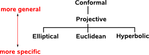
There are different ways to think about projective geometry:
- As a more general case of Elliptical, Euclidean and Hyperbolic geometries which can represent the properties of all of these. That is it has the same symmetries as the individual geometries with additional symmetries.
- As a geometry in n+1 dimensions with with the additional dimension added to allow us to represent points at infinity without the need to use the ∞ symbol. This can be important, for instance, any two lines will meet at a point and we don't have to make an exception for parallel lines.
- As a representation of perspective drawing.
This has many applications including:
- Projecting a 3D scene onto a 2D screen (used by openGL).
- Representing isometries (translations and rotations) as a single multiplication operation. This can greatly simplify the representation of objects moving in space.
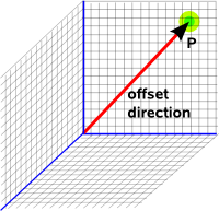
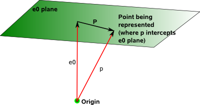
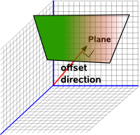
- Geometric algebra provides a powerful way to represent lines, planes, etc. which go through the origin, projective geometry provides a way to represent quantities offset from the origin.
- We can combine quantities to give 'meet' and 'join'.
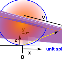
In the projective domain the length of the vector is less important because the projection onto the euclidean domain depends on the direction of the vector and not its length. There are different ways to deal with this redundant information regarding the length of the vector in the projective plane. Two of these models, the hemisphere model and the stereographic model are described below.
Results
Before we delve into the theory, here is a summary of some of the useful results, so that we know where we are heading.
There are different models for projective space, that is different ways to map between projective space and euclidean space:
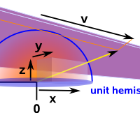
- hemisphere model - constrains projective space coordinates to unit sphere at origin: x² + y² + z² = 1
- stereographic model - constrains projective space coordinates to unit sphere at z=1: x² + y² + (z-1)² = 1
| hemisphere model | stereographic model | |||||||||||||||||||
|---|---|---|---|---|---|---|---|---|---|---|---|---|---|---|---|---|---|---|---|---|
 |
 |
|||||||||||||||||||
| euclidean coordinates to projective coordinates |
|
|
||||||||||||||||||
| projective coordinates to euclidean coordinates |
|
|
||||||||||||||||||
| infinity | a line for 2D case | a single point (0,0,0) | ||||||||||||||||||
| angles preserved (conformal) | no | yes | ||||||||||||||||||
| area preserved | no | no | ||||||||||||||||||
| results derived for 2D case: | on this page | on this page |
where:
- (u,v) = euclidean coordinates
- (x,y,z) = projective space coordinates
Relationship between hemisphere and stereographic model
The angle associted with the hemisphere model is half the corresponding angle in the stereographic model (as shown in trig identities page).
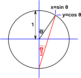
So, for instance, infinity is round the equator (90°) in the hemisphere model but it is the south pole (180°) in the stereographic model.
Representing Isometries
Projective space provides a way for us to represent movements of solid bodies in 3D space. If we want to model the movement of solid bodies using a computer then it is useful to be able to calculate the effect of a sequence of translations and rotations (such as a rotation about a point other than the origin) and to represent this combined transform as a single entity without the need to change the frame of reference or anything like that between rotations and translations. We have to pay a price for this which is that we have to increase the dimension of our quantities by one and map 3D, Euclidean Space to 4D projective space.
As we saw on this page, there is a 1:1 equivalence (a morphism) between the rotation of a 3D rigid body and the movement of a shape on the surface of a sphere. So calculation of 3D rotations using linear algebra becomes equivalent to mapping a flat Euclidean space to a curved spherical space. We are now stepping up a dimension and mapping 3D, Euclidean Space to 4D projective space.
| 3D Euclidean | 4D Projective | Matrix Notation | ||||||||||||||||
|---|---|---|---|---|---|---|---|---|---|---|---|---|---|---|---|---|---|---|
| vector[x,y,z] |
|
|||||||||||||||||
| point [x,y,z] | vector (depends only on direction not length of vector) |
|
||||||||||||||||
| line | bivector | ? | ||||||||||||||||
| translation |
|
|||||||||||||||||
| rotation |
|
|||||||||||||||||
| frustum projection |
|
One Dimensional Case
To represent 'n' dimensions we use 'n+1' dimensions in projective space. So lets start with a one dimensional case which will be represented as a two dimensional projective space. This one dimensional case may not have much practical application but it should allow us to establish the principles as simply as possible.
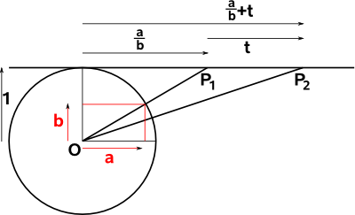
In the diagram above the horizontal line represents the one dimensional space. Points on the line, for example P1 and P2, are represented by the intersection of the horizontal line with a line from the origin O.
So, for instance, the point P1 can be represented by the line from 'O' the origin (the one dimensional space is offset from the origin by one unit).
This line can be represented by its normalised coordinates (a;b), that is the coordinates on the unit circle, although any scale factor 's' which gives (a*s;b*s) does not change the point as it still lies along the O to P1 line. So we can represent P1 by the ratio a/b.
One Dimensional transforms
In one dimension we don't have rotations so lets investigate translations. In the diagram above we want to translate P1 by 't' to P2. Of course we can do this by adding 't' as shown on the diagram but can we apply a transform using a multiplication? This would be useful when we move to higher dimensions and we want to combine translations and rotations.
We know that we can combine rotations using multiplication as described here so can we rotate the O to P line to perform a translation? As we can see from the above diagram this would not be linear because points nearer to 'O' would move more than points further away. Is it possible to use a different type of rotation such as hyperbolic rotation to perform our translation?
|
= |
|
|
Although this approximates projective transforms at small angles it does not work because projective geometry is represented by a shear transform, in order to represent translation by a rotation we need to use a conformal geometry.
Projecting onto a Line
Projecting a plane onto a line is discussed on this page.
To project points on the projective plane onto the line we can use the linear transform:
|
= |
|
|
where:
x'/y' = (m00 x/y + m01)/(m10 x/y + m11)
Algebra of One Dimensional Projective Space
We will start by using matrix algebra and then we will investigate using geometric algebra.
So in matrix and vector we can represent a point in projective space along the line we are using (which is offset by 1) as:
| p |
| 1 |
The transform is represented by this matrix:
| 1 | t |
| 0 | 1 |
This is a shear (also known as skew) matrix.
Multiplying them together gives the offset as required.
|
= |
|
|
Note that in projective space points (meaning location) and translations are represented by different types (unlike vector algebra) this is reasonable as they are different entities.
So we now have a way to perform a translation using multiplication, but at a cost, we are using a shear transform which is non-linear unlike say a rotation.
Combining Translations
If we want to combine two translations t1 and t2 then we can multiply their matrices together to give the required result:
|
= |
|
|
Homogeneous Coordinates in One Dimension
In the above notation we don't yet have the ability to represent points at infinity, so instead of representing the location by 'p' we will instead represent it by a/b in matrix notation our location is represented by:
| a |
| b |
So, for instance, zero will be:
| 0 |
| 1 |
and infinity will be:
| 1 |
| 0 |
The transform is now represented by this matrix:
| 1 | t/b |
| 0 | 1 |
Multiplying them together gives the offset as required:
|
= |
|
|
So the transform depends on the how the location (a;b) is scaled or normalised? Also combining transforms appears to be more complicated if they are normalised differently.
Shear Transform
Shear (also known as skew) transforms can be represented as a linear transforms, that is we can apply the transform by using a multiplication. However it is easier to represent shear transforms using matrices than Geometric Algebra. In order to use Geometric Algebra we may have to revert to using addition but Geometric Algebra has other advantages such as computing 'meet' and 'join'.
The determinant of shear transforms is 1, for instance,
det |
|
=1 |
Overview
It is an important subject because its used when we are representing a 3D world on a 2D plane in a way that it appears to our eye. For instance: horizontal lines appear to meet at the horizon. For an application of this see OpenGL pages. Projective transforms and the Möbius transform are also important in physics for instance: Roger Penrose uses the stereographic projection to analyze relativity.
For more information about the Möbius transform see this page.
This uses a 4D space to model the 3D world, the additional dimension gets round some problems we have when using the usual 3D vector space. The extra dimension can be thought of as the point at the origin in the physical space.
This space, known as Projective Space, allows us to represent a location in physical space as a direction (ratio of x,y,z with w). Since rotations operate on directions then this gives us a way to represent rotations and translations in a common way.
It is useful where:
- we want to model both rotations and translations in a single operation.
- we are projecting 3D models onto a 2D screen.
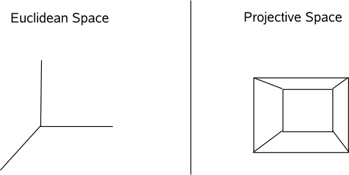
Projective Space
This is used as the coordinate system for projective space. Projective space has one additional dimension compared to the equivalent euclidean space.
This page discusses rendering 3D models on a 2D screen.
| (x,y,z) | (x:y:z:w) |
Plücker Coordinates
If a point is at (x,y,z) in euclidean space then the equivalent in projective space is (x*w, y*w, z*w, w). Or to put it the other way round, if a point is defined as (x',y',z',w) in projective space this is equivalent to (x'/w,y'/w,z'/w) in euclidean space. So we can scale the object in projective space without affecting what it represents.
more about Plücker coordinates here.
We can also use Geometric Algebra or Matrices to represent the homogeneous geometry.
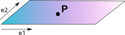
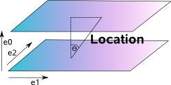
Geometric Algebra Representation
Here we can see how we represent a location in physical space as a direction (ratio of x,y,z with w) in homogeneous space
| quantity | Physical Space | Homogeneous Space |
|---|---|---|
 |
 |
|
| coordinate | x,y,z | x,y,z,w |
| direction | a (notation as bold) |
a |
location |
a = vector (representing an offset from origin) |
a + e0 |
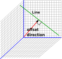
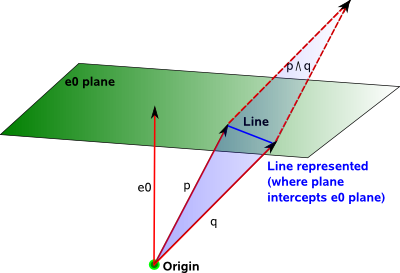
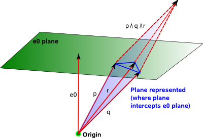
| oriented line | outer product of two vectors: a^b |
|
| oriented plane | outer product of three vectors: a^b^c |
|
For a discussion of alternative ways to use Geometric Algebra to combine rotations and translations see this page.
This geometric algebra has 4 dimensions (which all square to +ve), known as G4,0,0, this is discussed on this page. We could alternatively allow e0 to square to -ve, this would work just as well.
One of the advantages of projective space is that it allows points at infinity to be defined. The plane at infinity is identified by (x,y,z,0).