Cell Complexes

There are many ways to approach cell complexes. They originally arose from topology but they can also be used in a purely combinatorial context or an algebraic context. We can also look at them as a generalisation of the structure of a graph.

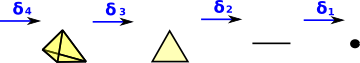
A simplex is a simple shape, called a face, such as a point a line a triangle a tetrahededron ...

These faces can be glued together, in ways discussed here, to form complex shapes.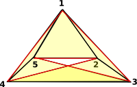

Building Complex Shapes

There are different ways to specify which simplicies are glued together to produce a complex shape. One way is to name all the points in the complex (in this case 0, 1, 2 and 3) and then define the higher dimensional faces in terms of these names.

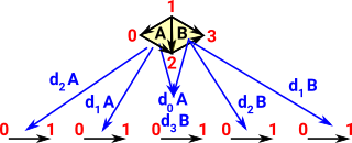Another way is to name the highest dimensional faces (in this case triangles A and B) then specify the sub-faces using face maps (explained later). Then we can use equations to specify the faces glued together (for example here d0A=d3B)

There is two types of structure here:

• The subface structure within a simplex - This will always be the same for a given simplex such as a triangle.
• The sub structure within a complex - This will depend on the shape which faces we need to glue together.

Simplicial Complexes

In a graph an edge has arrows to two vertices (the source and target). Simplicial complexes generalise this to allow any number of vertices.

Introduction

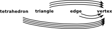
A 'simplex' is a set of vertices such that every subset is included in the simplex. For example a tetrahedron contains all its faces and lines.

A 'simplicial complex' is a set of these simplexes which may have vertices in common.

Because each simplex contains its subsets this is a combinatorial structure, when used in this way the structure is known as an 'abstract simplicial complex' optionally we can also associate a point in a space with each vertex, in this case the structure is known as an 'geometric simplicial complex' and it has geometric/topological/homotopy properties.

Representation

The representation holds whole Simplicial Complex. This consists of a vertex set, represented as a vertex list so that we can index it. Also a list of simplices (that is n-dimensional faces). each simplice is an array of vertex indexes. So each simplice is a subset of the vertex set.

If the dimension given for the simplicial complex is 'k' then:

• The number of elements in each vertex = k.
• The maximum number of vertexes in each simplice = k + 1.

For example, a triangle has 3 vertexes, so it is maximum size face in 3-1=2 dimensions.

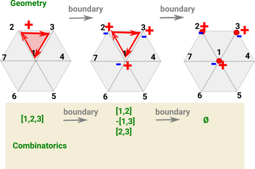
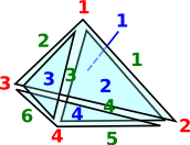
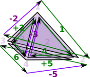
Combinatorics

Here we choose the labeling of the points, lines, triangles and so on to show the combinatorics aspects. Instead of giving each dimenstion its own labeling scheme we choose a labeling scheme that illustrates the relationship between the dimensions.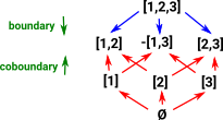

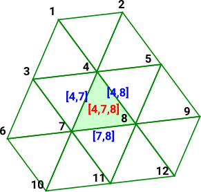
Homology Homology is point-centric in that we start with the points and the arrows go up to the higher dimensions. So here I have labeled the points by a single index, each line is labeled by a list of the two points it connects, the triangles by 3 indices, and so on. (for now I have not specified the orientation). If there were two lines between the same points then it would be unclear how to uniquely label each line.
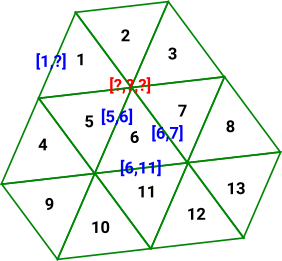
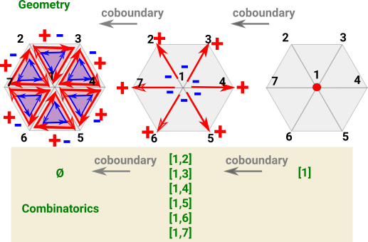
Cohomology Cohomology starts with the higher dimensions and the arrows go down to the points. So here I have labeled the triangles with a single index and tried to relate this down the dimensions. The lines have two indices relating a common edge of two triangles, This works on a continuous surface but it is unclear how to label a boundary edge. Also it is unclear how to label points since, in this case, they join 6 triangles but we only need 3 to specify the point.
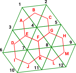
Poincaré Duality Perhaps to get poincaré duality we need to go from triangles to hexagons?

So, for now, concentrate on the homology case:

We can identify the n-dimensional simplices (line, triangle ...) by the points they contain.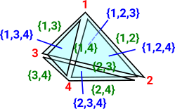
The relations are shown more clearly in an attachment diagram here. This shows subset relations with the arrows going from lower dimension to higher dimension.

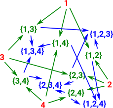Sheaf

A sheaf assigns some data spaces to the attachment diagram above. In this case reals (ℜ) - A sheaf of vector spaces. Each such set is called a stalk over the simplex. ℜ in all the points gives a vector ℜ² a matrix links the vectors, each such function is known as a restriction.

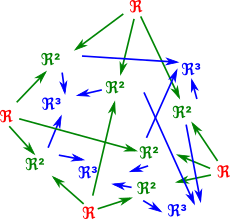Section - an assignment of values from each of the stalks that is consistent with the restrictions.

Sections can be:

• Global - defined everywhere.
• Local - defined for some part.

If all local sections extend to global sections the sheaf is called flabby/flasque (don't have interesting invariants).

More about sheaves on this page.

Delta Complex

The above representation defines faces, of any dimension, by their vertices. This can be an efficient way to define them, but sometimes we need to define each dimension in terms of the dimension below it, for example, when generating homotopy groups such as the fundamental group.

To do this we represent the complex as a sequence of 'face maps' each one indexed into the next.

This is an alternative way to represent simpectial complexes, in most (but not all) cases the representations are isomorphic.

As an example consider the representation for a single tetrahedron:

The usual representation would be:	(1,2,3,4)
which is very efficient but it does not allow us to refer to its edges and triangles.
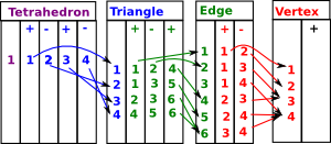
Here we have indexed: The 4 vertices (in red) The 6 edges (in green) The 4 triangles (in blue)
This representation holds all these indexes so that we don't have to keep creating them and they can be used consistently.
Face Maps So the tetrahedron indexes its 4 triangles, each triangle indexes its 3 edges and each edge indexes its 2 vertices. Each face table therefore indexes into the next. To show this I have drawn some of the arrows (I could not draw all the arrows as that would have made the diagram too messy).

Since edges, triangles, tetrahedrons, etc. are oriented we need to put the indexed in a certain order.

Edges are directed in the order of the vertex indices. That is low numbered index to high numbered index: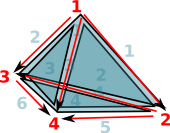
For triangles we go in the order of the edges, except the middle edge is reversed. On the diagram the edges are coloured as follows: green arrows - not reversed purple arrows - reversed This gives the triangles a consistent winding
However the whole tetrahedron is not yet consistent because some adjacent edges go in the same direction and some go in opposite directions.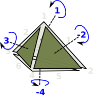
This gives the orientation of the faces as given by the right hand rule. That is: if the thumb of the right hand is outside the tetrahedion, pointing toward the face, then the fingers tend to curl round in the direction of the winding.

I have put more information about delta complexes on the page here.

Abstract Simplicial Complex vs. Geometric Simplicial Complex

If we apply the restrictions explained so far we have an abstract simplicial complex, However, for a geometric simplicial complex there are some additional conditions.

The additional tests for a geometric simplicial complex are described on the page here.

An Abstract Simplicial Complex is purely combinatorial, that is we don't need the geometric information.

Therefore the AbstractSimplicialComplex domain does not need coordinates for the vertices and they can be denoted by symbols.

Simplicial Maps

Allow edges to be collapsed into vertices.

Oriented Simplexes Maps

Because the code uses Lists instead of Sets the simplexes are oriented by default, if that is not needed then we can just ignore the order.

Topological Aspects of Simplicial Complexes

We implement topological aspects of simplicial complexes such as boundaries and cycles. The code for this is explained on the page here.

Operations on Simplicial Complexes

• Closure - closure of X contains X and all the faces touching X
• Star(A,b) -set of sub-simplices of 'A' which contain face 'b'.
• Link - The 'link' of a simplicial complex and a vertex contains
  the boundary of the simplexes of s which include simplex.
• Join - We will call it a SimplicialJoin since it is not related to joins in lattices.
• Products are quite complicated so I have put this on a separate page here.

Here are some examples, first we setup some simplicial complexes to work with:

(1) -> ASIMP := FiniteSimplicialComplex(VertexSetAbstract)
   (1)  FiniteSimplicialComplex(VertexSetAbstract)
                                                                   Type: Type

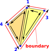
(2) -> v1:List(List(NNI)) := [[1::NNI,2::NNI,3::NNI],[4::NNI,2::NNI,1::NNI]]
   (2)  [[1,2,3],[4,2,1]]
                                         Type: List(List(NonNegativeInteger))

(3) -> sc1 := simplicialComplex(vertexSeta(4::NNI),v1)$ASIMP

   (3)
        (1,2,3)
        (1,2,4)
                             Type: FiniteSimplicialComplex(VertexSetAbstract)

(4) -> v2:List(List(NNI)) := [[1::NNI,2::NNI]]
 

   (4)  [[1,2]]
                                         Type: List(List(NonNegativeInteger))
(5) -> sc2 := simplicialComplex(vertexSeta(2::NNI),v2)$ASIMP

   (5)
        (1,2)
                             Type: FiniteSimplicialComplex(VertexSetAbstract)

Now we can calculate a boundary. Note that this corresponds to the red line on the diagram above, that is, the boundary.

(6) -> delta(sc1)$ASIMP

   (6)
         -(1,3)
         (2,3)
         (1,4)
         -(2,4)
                             Type: FiniteSimplicialComplex(VertexSetAbstract)

Now we can test star,join and link

(7) -> star(sc1,orientedFacet(1,[4]))

   (7)
        -(1,2,4)
                             Type: FiniteSimplicialComplex(VertexSetAbstract)
(8) -> link(sc1,orientedFacet(1,[4]))

   (8)
        -(1,2)
        (1,4)
        -(2,4)
                             Type: FiniteSimplicialComplex(VertexSetAbstract)
(9) -> cone(sc1,5)

   (9)
         (1,2,3,5)
         (1,2,4,5)
                             Type: FiniteSimplicialComplex(VertexSetAbstract)
(10) -> delta(sc2)$ASIMP

   (10)
         (1)
         -(2)
                             Type: FiniteSimplicialComplex(VertexSetAbstract)
(11) -> simplicialJoin(sc1,sc2)

   (11)
         (1,2,3)
         -(1,2,4)
          (1,2)
                             Type: FiniteSimplicialComplex(VertexSetAbstract)

We can also calculate products and sums of simplicial complexes. Products are quite complicated so I have put this on a separate page here.

Vertex Set Code

We want an indexed set of points, the simplest way to do the indexing is to use 'List' instead of 'Set'.

The vertices themselves may be either:

• literal coordinates.
• symbolic vertex names.
• numeric indexes.

So we cave a category that can represent any of these types and then a domain for each type.

Algebraic topology turns topology problems into algebra problems.

As discussed on an earlier page, in two dimensions it is relatively easy to determine if two spaces are topologically equivalent (homeomorphic). We can check if they:

• are connected in the same way.
• have the same number of holes.

However, when we scale up to higher dimensions this does not work and it can become impossible to determine homeomorphism. There are methods which will, at least, allow us to prove more formally when topological objects are not homeomorphic.

These methods use 'invariants': properties of topological objects which do not change when going through a homeomorphism.

An important invariant is the number of 'holes' in each dimension.	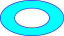Here there is one hole, any homeomorphic transformation will still have one hole.
Dually we could look at the maximum number of n-dimensional cuts we can make without dividing into two. This is really the same thing since each cut removes a hole.	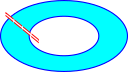This cut does not divide the shape into two parts because we can still go round the other way.

If the above invariants are the same it is a good indication that the shapes are homeomorphic but it is not enough, other factors like 'torsion' also need to be unchanged to be sure.

Here we look at two types of invariants which arise from homotopy and homology. (I have written some code to implement these structures on the page here)

These invariants can be expressed as algebraic structures, particularly groups, so this subject is called 'algebraic topology'. The way that these algebraic structures arise is discussed on the homotopy and homology pages but first we need to introduce a way to specify topological objects in a way that we can calculate with. We will do this by using simplicial complexes.

Equivalance Classes

Equivalance classes exist when we have classes we wish to consider essentially the same.

Examples:

• A set of objects with the same shape.
• The set of integers with the same remainder when divided by a given number.

So we can start to get the idea that this is related to the concept of quotient.

An equivalence relation has the following properties:

• reflexive
• symmetric
• transitive

See partial order for more.

Homotopy and Homology Equivalance

In the homotopy case we have path components of X written π(X)

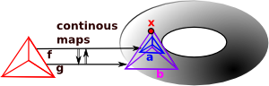
We have a continuous map from space X to space Y: f: X -> Y and a continuous map from space Y to space X: g: Y -> X

Homotopy

A homotopy is a continuous mapping between two spaces. Often parameterised by 't' to be though of as time.

Homotopy Groups

The fundamental group of a pointed space (mostly represented here by simpectial complexes) is isomorphic to the fundamental group of the space (Seitert-Van Kampen theorem).

We look at loops of maps from a point to the given space. Each loop, in the space, from the point back to itself is a generator for the group. These loops can then be composed. The homotopy group is is finitely presented by generators and relations. This representation of a group is not, in general, algorithmically computable into other representations of a group.

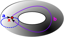The simplest homotopy group is the fundamental group. It determines when two paths, starting and ending the point, can be continuously deformed into each other. It records information about the shape in terms of holes in the topological space.
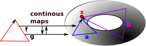nth homotopy group. Instead of mapping a circle onto our topological space we map a sphere or higher order sphere onto the space.

To generate the fundamental group from the simplicial complex see the page here.

Homology

When we looked at the delta complex we got a chain of 'face maps' between each dimension and the next lower one.

In homology we treat this as a chain of abelian groups.

More detail on the page here.

Next Steps

• The additional tests for a geometric simplicial complex are described on the page here.
• The way we implement topological aspects of simplicial complexes such as boundaries and cycles is explained on the page here.
• To generate the fundamental group from the simplicial complex see the page here.
• Products are quite complicated so I have put this on a separate page here.

Bibliography

For more details see:

• [1] Mathematics++ Kantor,Matousek,Samal 2015 ISBN 978-1-4704-2261-5 Chapter 6 - Topology. Contains a relatively gentle introduction to homology.
• [2] Graphs, Surfaces and Homology, Peter Giblin 2010 ISBN 987-0-521-15405-5
  Builds up to homology groups via graphs and simplicial complexes.
• [3] Wikipedia
• [4] How to compute this stuff
• [5] Hatcher - Algebraic Topology - book also available free online.
  

EuclideanSpace

home

Where Are You

This is one of a series of pages about topology, these pages start here.

On these pages we discuss some concepts of topology:

• Open Sets
• Fibre bindles
• Algebraic Topology
  • Simplicial Complexes
  • Delta Complexes
  • Chains
  • Homology
  • Homotopy

Computer Code Implementation

I have written some code to implement algebraic topology structures. For an explanation of this code see the page here.

Comparison of Model Category and Set Category

Model categories are introduced on page here.

	Set Category	Model Category
Objects In category theory set objects are often thought of as 'n' elements without any further structure (just an unconnected set of points) or empty set. In model theory objects are spaces, say a topological space with a subobject structure.
Morphisms In both cases mappings can be decomposed into 3 types:	bijections	weak equivalences
	surjections reversing this leads to fibre bundles	fibrations
	inclusions reversing this leads to equivilance classes and logic.	cofibrations

For more comparison of model category and set category see page here.

Homology

Algebraic Topology

Fibration and Co-fibration

Homotopy has the concept of:

• a fibration which has the lifting property.
• a co-fibration which has the extension property -extension is dual to lift.

Kan fibrations are combinatorial analogs of Serre fibrations of topological spaces.