Simulation using discreet step integration
This page shows methods to calculate the motion of a solid object, or a systems of objects, assuming that we know, or can calculate, the forces and impulses on those objects. To calculate the position and orientation from the forces first involves an integration to get to the velocity and then another integration to get the position and orientation. If the object is not rotating and if the forces on it are constant then it is relatively easy to derive an equation to give the objects position at any given time as shown on the kinematics page here.
If the object is rotating and if the forces on it are varying with time then, the equations to specify its position and orientation for any given time will rapidly get more complicated and harder to derive. Therefore, for most simulations, other than the simplest possible, we need to find another way to do these integrations.

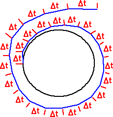
The discreet step integration method, calculates the next position from the current position and the forces at the time, this fits quite well with animation because we need to display or render the scene regularly to give the viewer the correct sense of movement, so we can do the physics calculations in the render loop. However we need to be careful, using a finite time interval is an approximation and inaccuracy can build up over time. The error depends on both the time step size and the nature of the simulation, some types of model would not be very appropriate for this method, for example say we were modeling a planet orbiting the sun, after a while the errors would start to build up, getting worse until the planet spins off to infinity. However, most interactions in games could be modeled accurately enough to look right.

So at each frame, and for each object, we need to do the following steps:
- Calculate the net forces and torques acting on the object.
- From this we can calculate the acceleration and angular acceleration of the object.
- From this we can calculate change in velocity and angular velocity of the object, use this to update the current velocity and angular velocity.
- If there is a collision calculate and add in the change in velocity and angular velocity due to impulse.
- From this we can calculate change in position and orientation of the object, use this to update the current velocity and angular velocity.
Method using Matrices to represent rotations
Using the method described by Chris Hecker.
See here http://www.d6.com/users/checker/pdfs/gdmphys4.pdf
This paper starts by describing some concepts like axis and angle, but by the time it gets to this algorithm for solid body movement it skips some of the details, so I have tried to fill in some of the gaps here:
Note: in some cases I have used a slightly different notation to show which quantities are scalars, vectors and matrices, functions of time are shown as f(t) or f(n) as we are using discreet time intervals..
Initialisation - set the following quantities before the simulation begins
| [I]-1 |
Calculate the Inverse of Inertia Tensor - Calculate the Inertia Tensor about the centre of mass in local co-ordinates, if we don't have details of the objects mass distribution we might be able to approximate it from the geometry co-ordinates. We then find the inverse of the matrix. It will simplify the calculations if the local co-ordinate system has been chosen so that [I] is a diagonal matrix. For more information about Inertia Tensor see here. |
| M | The mass is a fixed scalar quantity that we need to know. |
| Set initial position vector , in other words the position of the centre of mass at the first frame. See position | |
| Set initial velocity, in other words the velocity at the first frame. See velocity | |
| [R(0)] |
Set the initial local to world transformation. I have used the notation
[R] to show that it is a rotational matrix, i.e. a 3x3 orthogonal matrix.
We could use a 4x4 matrix to combine both the rotational and translational
components, but that will complicate some of the calculations, for example
to calculate [I] in world co-ordinates, so it may be best to leave [R]
and There are other possibilities for representing orientation, such as quaternions, for information about representing orientation see here. |
| Set the initial angular momentum, we need to know either the initial angular momentum or the initial angular velocity, we can calculate one from the other using L=Iw | |
| Auxiliary quantities | |
| [Ia(0)]-1 = [R(0)][I]-1[R(0)]-1 | Calculate the Inverse of Inertia Tensor in absolute world co-ordinates |
| If we have not calculated the initial angular momentum from the initial angular velocity, then we can calculate the initial angular velocity from the initial angular momentum |
Simulation:
This part is done once for every frame, it could be part of the render loop:
| Compute individual forces, forces happen in pairs see here. | |
| Compute the application points of each of the individual forces above | |
| h | set h to the time since the last frame. |
| Integrate | |
| integrate velocity - add change in velocity calculated from
|
|
| integrate position - add change in position of centre of mass | |
| [Ia(n+1)]-1 = [R(n)][I]-1[R(n)]-1 |
calculate inertia tensor in world coordinates Since [R(n)] is orthogonal we can use [R(n)]-t instead of[R(n)]-1 |
| integrate angular momentum, uses |
|
| calculate angular velocity from angular momentum | |
| [R(n+1)] = [R(n)] + h [~w][R(n)] |
integrate orientation Multiplying by tilde
matrix [~w] is the equivalent of cross multiplying by the [ so the equation is really [R(n+1)] = [R(n)] + h [ I can see what this saying, the change in matrix values is the rate of change times delta t, but I'm still uneasy about adding rotation matrices in this way? normally if we want to apply subsequent rotations then we multiply the rotation matricies. I would really like more theoretical underpinning for this. |
|
reorthogonalize [R(n+1)]
|
Correct for the error introduced above - see here for orthogonal matrix To do this we multiply it by C, where: [C] = (3[I]-([M] * [M]T))/2 this is explained here |
| collision | |
| test for collision. see collision detection | |
|
if collision apply impulse to both colliding objects.
|
if collision detected calculate impulse
|
Thank you Todd for
helping me with this
Possible Method using Quaternions to represent rotations?
The result of combining rotations can be calculated by either 3x3 orthogonal matrix multiplication or quaternion multiplication. When used in this way 3x3 orthogonal matrices and quaternions are equivalent. Since quaternions have less redundancy (4 numbers as opposed to 9) it seems like it might be a good idea to use quaternions instead of matrices. The problem is that the inertia matrix can't be represented by quaternions (as shown on this page). So is there a way to use quaternions to represent the rotations but still use a matrix for the inertia tensor? We can use quaternions to represent the rotational quantities such as torque and angular acceleration, is there any way we could use a 4x4 matrix to translate directly from one quaternion to another?
Initialisation - set the following quantities before the simulation begins
| [I]-1 |
Calculate the Inverse of Inertia Tensor - Calculate the Inertia Tensor about the centre of mass in local coordinates, if we don't have details of the objects mass distribution we might be able to approximate it from the geometry coordinates. We then find the inverse of the matrix. It will simplify the calculations if the local coordinate system has been chosen so that [I] is a diagonal matrix. For more information about Inertia Tensor see here. |
| M | The mass is a fixed scalar quantity that we need to know. |
| Set initial position vector , in other words the position of the centre of mass at the first frame. See position | |
| Set initial velocity, in other words the velocity at the first frame. See velocity | |
| Q(0) |
Set the initial local to world transformation. I have used the notation Q to show that it is a quaternion. |
| Set the initial angular momentum, we need to know either the initial angular momentum or the initial angular velocity, we can calculate one from the other using L=Iw | |
| Auxiliary quantities | |
| [Ia(0)]-1 = Q(0)[I]-1Q(0)-1 | Calculate the Inverse of Inertia Tensor in absolute world coordinates |
| If we have not calculated the initial angular momentum from the initial angular velocity, then we can calculate the initial angular velocity from the initial angular momentum |
Simulation:
This part is done once for every frame, it could be part of the render loop:
| Compute individual forces, forces happen in pairs see here. | |
| Compute the application points of each of the individual forces above | |
| h | set h to the time since the last frame. |
| Integrate | |
| integrate velocity - add change in velocity calculated from
|
|
| integrate position - add change in position of centre of mass | |
| [Ia(n+1)]-1 = Q(n)[I]-1Q(n)-1 |
calculate inertia tensor in world coordinates
|
| integrate angular momentum, uses |
|
| calculate angular velocity from angular momentum | |
| Q(n+1) = Q(n) + h 0.5 qw Q(n) |
integrate orientation Q(n+1) = Q(n) + h [dQ/dt] where
see derivation for dQ/dt here |
| normalise Q(n+1) | Correct for the error introduced above |
| collision | |
| test for collision. See collision detection | |
|
if collision apply impulse to both colliding objects.
w(n+1) = [Ia(n+1)]-1 angular impulse |
if collision detected, calculate impulse
|
Next Step and Further Reading
We now want to go on to implement this method to simulate physical objects using our program. The first stage is to define a data structure for storing this information, this is discussed here.
