| When we looked at the delta complex we got a chain of 'face maps' between each dimension and the next lower one. | 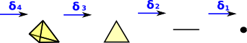 |
| For cochain we reverse the arrows: | 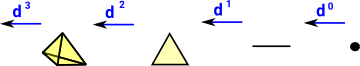 |
As with the chain (see previous page) we represent each one of these mappings with a matrix. For a cochain this matrix is transposed compared to the chain.
FriCAS Implementation
| In the following example we create a shape (triangle) with 3 points. We then associate a value (in this case an integer) to each of these points: |
|
The coboundary function then calculates the differences: [1,2,1]. That is the difference between 3 and 4 is 1, the difference between 3 and 5 is 2, and the difference between 4 and 5 is 1.
When we apply the coboundary function again we get the difference around the loop, that is, 0.
| For comparison, first generate a chain. | (1) -> FACTORY := _
SimplicialComplexFactory(Integer)
(1) SimplicialComplexFactory(Integer)
Type: Type
(2) -> b1 := sphereSolid(2)$FACTORY
(2) points 1..3
(1,2,3)
Type: FiniteSimplicialComplex(Integer)
(3) -> d1 := deltaComplex(b1)
(3)
2D:[[1,- 2,3]]
1D:[[1,- 2],[1,- 3],[2,- 3]]
0D:[[0],[0],[0]]
Type: DeltaComplex(Integer)
(4) -> c1 := chain(d1)
+ 1 1 0 + + 1 +
(4) [0 0 0],|- 1 0 1 |,|- 1|,[]
+ 0 - 1 - 1+ + 1 +
Type: ChainComplex
|
| The cochain has the reverse order and the matrices are all transposed | (5) -> cc1 := coChain(d1)
+1 - 1 0 + +0+
(5) [],[1 - 1 1],|1 0 - 1|,|0|
+0 1 - 1+ +0+
Type: CoChainComplex(Integer)
|
| We associate integer values, one for each point. The coboundary function takes these values and calculates the differences. | (6) -> cb1 := coboundary(cc1,2::NNI,_
[3::Integer,4::Integer,5::Integer])
(6) [1,2,1]
Type: List(Integer)
(7) -> cb2 := coboundary(cc1,3::NNI,cb1)
(7) [0]
Type: List(Integer) |
The values used here were Integers but we could use any type that implements AbelianGroup.
For example we could have real (Float) values associated with each point representing say voltage or height or some other quantity for each point.
Perhaps the most obvious quantity we could associate with each point is position, given by a vector relative to some origin and coordinate system. However the type (domain) needs to implement AbelianGroup. Unfortunately Vectors in FriCAS don't implement AbelianGroup because it needs to implement 0:% which it can't because the nearest function in Vector is zero: NonNegativeInteger -> % but this needs to know the number of dimensions.
What is needed is a version of Vector which has the number of dimensions built in to the type (as a type parameter) rather than having a variable dimension. This could then implement AbelianGroup.
(8) -> P1 : DirectProduct(3,DoubleFloat) := _
     construct([1.2,3.4,6.7])$(Vector DoubleFloat)

   (8)  [1.2,3.4,6.699999999999999]
              Type: DirectProduct(3,DoubleFloat)
(9) -> P2 : DirectProduct(3,DoubleFloat) := _
     construct([1.9,3.2,6.0])$(Vector DoubleFloat)

   (9)  [1.9,3.2,6.0]
              Type: DirectProduct(3,DoubleFloat)
(10) -> P3 : DirectProduct(3,DoubleFloat) := _
     construct([1.7,3.8,6.9])$(Vector DoubleFloat)

   (10)  [1.7,3.8,6.9]
              Type: DirectProduct(3,DoubleFloat)
(11) -> FACTORY2 := SimplicialComplexFactory(_
            DirectProduct(3,DoubleFloat))

   (11)  SimplicialComplexFactory(DirectProduct(3,DoubleFloat))
                                      Type: Type
(12) -> b2 := sphereSolid(2)$FACTORY2

   (12)  points 1..3
           (1,2,3)
                  Type: FiniteSimplicialComplex(DirectProduct(3,DoubleFloat))
(13) -> cc3 := coChain(b2)

                        +1  - 1   0 + +0+
                        |           | | |
   (13)  [],[1  - 1  1],|1   0   - 1|,|0|
                        |           | | |
                        +0   1   - 1+ +0+
                           Type: CoChainComplex(DirectProduct(3,DoubleFloat))
(14) -> lab : List(DirectProduct(3,DoubleFloat)) := [P1,P2,P3]

   (14)  [[1.2,3.4,6.699999999999999],[1.9,3.2,6.0],[1.7,3.8,6.9]]
        Type: List(DirectProduct(3,DoubleFloat))
(15) -> cb3 := coboundary(cc3,2::NNI,lab)

   (15)
   [[0.7,- 0.19999999999999973,- 0.6999999999999993],
    [0.5,0.3999999999999999,0.20000000000000107],
    [- 0.19999999999999996,0.5999999999999996,0.9000000000000004]]
Type: List(DirectProduct(3,DoubleFloat)) |