Maths - Calculus

Definition of a function

If two variables x and y are so related that the value of y depends on the value of x, y is said to be a function of x.

Examples of functions:

• y = 3x² + 2x + 4
• y = log_e x
• y = sin² x

The statement y is a function of x can be stated y=f(x), the term inside the bracked defines the specific function.

Note: f(x) should not be regarded as the product of f and x.

Consider the function: y=1/x

As x increases y decreases, as y increases x decreases. Consider x having a value infinitely large i.e. (x approaches infinity ∞) y gets correspondingly smaller and approaches 0.

This can be stated: within the limit as x approaches ∞, y approaches 0.

Or limit_x-›∞(1/x)=0

Measurement of rate of increase

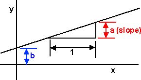
Consider the straight line graph :

y = a x + b

The slope or gradient = a

This could be stated: the rate of increase of y with respect to x = a

(increase in y) / (increase in x) = a

The rate of increase is constant because the graph is a straight line, for a curved graph the slope or gradient or rate of increase is varying.

Consider a graph of the form:

y = a x² + b x + c = 0

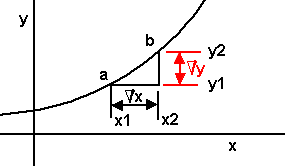
between 'a' and 'b' the rate of increase of y with respect to x = (increase in y) / (increase in x)

= (y2 - y1) / (x2 - x1)

This rate represents the average rate of increase between 'a' and 'b'.

Let:

• Δx = increase in x from a to b
• Δy = corresponding increase in y

(Note: Δ or DELTA is an operator which means a small increase or increment in the value of x and so d is not a variable and it does not mean Δ*x)

So,

Δx/Δy = (y2 - y1) / (x2 - x1)

which is the rate of increase in y with respect to x from a to b.

Although Δx and Δy are both small, Δx/Δy still represents the rate of increase between a & b. As b is moved closer to a & x becomes smaller and within the limit approaches 0. i.e. the gradient or rate of increase at the point 'a' is given by:

limit_dx-›∞(Δy / Δx)

which represents dy / dx.

dy / dx is known as the differential coeficient of y with respect to x and is the limiting value of the function Δy / Δx as Δx approaches 0.

Consider a graph y=x²

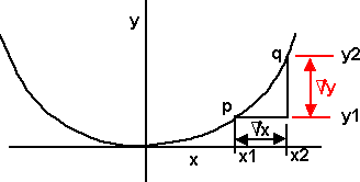
At the point p: y1 = x1²

At the point q: y1 + Δy = (x1 + Δx)²
y1 + Δy = x1² + 2xΔx + Δx²

subtacting gives:

Δy = 2xΔx + Δx²

divide by Δx:

Δy/Δx = 2x + dx

this gives the rate of change between p and q for any value of x

eg at x=3 then Δy/Δx = 6 + dx

if Δx = 0.5 Δy/Δx = 6.5

if Δx = 0.05 Δy/Δx = 6.05

if we take the limit as Δx tends to 0 then:

dy/dx = 2x

therefore 2x represents the gradient for any value of x

eg at x=3 gradient = 6

at x=-1 gradient = -2

Differentiation from first principles

Consider y = x² + 2

y + dy = (x + dx)² + 2
y + dy = x² + 2xdx + dx² + 2

subtacting gives:

dy = 2xdx + dx²

divide by dx:

dy/dx = 2x + dx

let dx -› 0

dy/dx = 2x

In general if:

y = a xⁿ

dy/dx = a n x^n-1

---

General Principles

In algebra an equation represents a precise quantitive relationship between an unknown quantity and one or more known quantities, in calculus, the unknown is not a single quantity but an entire function.

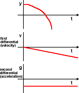
Differentiation turns a function into its rate of change, Integration is the inverse of this process.

Differential equations are important for simulating the physical world, examples are: change of position with time, and also the change of pressure with distance through an object. The first type tends to be solved using initial value information, the second type using boundary values. We will cover initial value solutions first, then boundary solutions, in both cases we will cover analytical and numeric methods.

Time varying position - initial value solutions

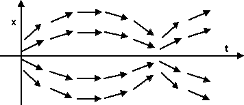
Equation depends on constraints and positions of forces, for example, if an object is constrained to move in the y-plane and if it is under a constant force then:

 

---

Examples from physics

Example 1 - acceleration under gravity

A mass accelerates under the influence of gravity. Due to Newtons second law (Force = Mass * Acceleration), the equations of motion tend to be expressed in terms of the second differential with respect to time, in this case this is a constant defined by the gravity constant.

So solving this example is just a case of integrating twice. We need to know the initial value conditions, for instance, the velocity and position at time=0.

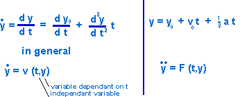
So in general the acceleration is some function of time and position: y'' = F(t,y)

In this case the acceleration (which is proportional to force) is constant. So the force field is as follows:

---

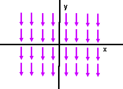
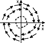
Example 2 - 1-dimensional oscillating spring

In this example a mass is free to move in the x direction, it is connected to a spring which generates a force toward a fixed point.

So the force field is as follows:

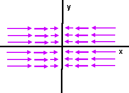
So there are two forces which must be equal, these are:

force = m x'' = - k x

so

x'' = f(t,x) = - k/m * x

 

 

---

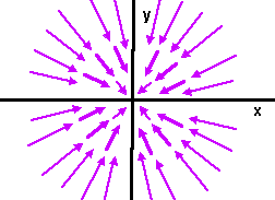
Example 3 - 2-dimensional orbiting mass

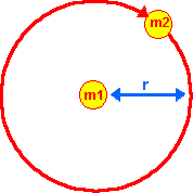
The acceleration of the mass m2 is inversely proportional to its distance from m1

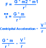
So the force field due to m1 is as follows:

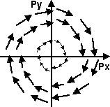
However there is also a force due to momentum (centripetal force) so the masses will tend to orbit each other.

---

Analytical Integration

Harmonic Oscillator

 

.	0	1
x =	-k/m	0	x

 

x	0	1	x
x	-k/m	0	x

 

x(t0) x
x = -k/m x

Jacobian Matrix

The Jacobian shows how a multidimensional function transforms an infinitesimal square (or cube, or hypercube, etc.)

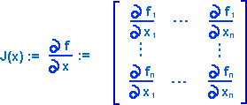
The Jacobian for a complex function is shown on this page.

---

Numerical Integration

Eulers Method

public void step() { 
	velocity.add(acceleration); 
	distance.add(velocity); 
	angularVelocity.add(angularAcceleration); 
	angularDistance.add(angularVelocity); 
}  

Runge-Kutta Method

Taylor series:

x(t0 + h) = x(t0) + h x'(t0) + h^2/2 x''(t0) + O(h^3).

EuclideanSpace

home

Trigonometry Functions

Standards