I think it may be worthwhile to take a bit of time to try to understand the geometry and graphics structures in axiom (for the reasons discussed on this page). I can't quite find the information I need, there is some documentation here:
- bookvolume0 - 7.2.6 - Building 3D primitives from scratch
- and HyperDoc - Topics->Graphics->
But it not quite what I need so I have been putting together this information gathered from what I can work out from the source code. Since I would like to use ThreeSpace and related domains to output graphical information to a file I need to understand them.
So here is what I have found so far, click on a structure in this diagram to link to the information on this page about it:
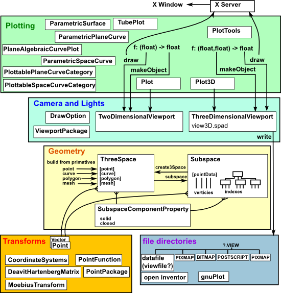
ThreeSpace
space.spad
I have put a tutorial on this page about how to create ThreeSpace from primitives or from draw or plots.
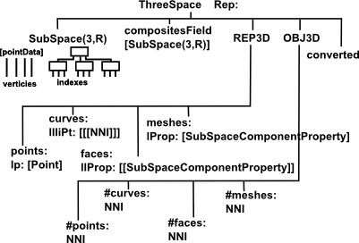
ThreeSpace is a domain which is a wrapper for SubSpace(3,R) geometry, that is a SubSpace which is 3D. Four dimensional points are also supported where the fourth dimension represents colour.
Once this 'SubSpace' geometry has been set from the SubSpace structure in this ThreeSpace domain then the domain can be 'converted' which means the raw geometry data is converted into separate information about:
- Points
- Curves
- Polygons
- Meshes
The domain stores the information in the following form:
SubSpace
newpoint.spad
SubSpace stores geometry information (limited to points, curves, polygons and meshes). Unlike ThreeSpace, SubSpace can support geometry in two dimensions as well as 3/4 dimensions. In the case of ThreeSpace then it contains the SubSpace structure.
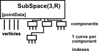
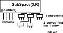
SubSpace is a tree structure where the leaves are indexes to Point (vertex) data, there are 3 layers in this tree, each of these layers contains SubSpace instances. I will follow the convention in the code and describe the layers as:
- components - contains a complete point,curve,polygon or mesh.
- curve - not just for a curve node but any substructure within a component.
- index - leaf node containing .
We can covert out geometric structure between the two structures using:
- subspace: (ThreeSpace) -> SubSpace
- create3Space : SubSpace(3,R) -> ThreeSpace
The point data is indexed so if a given point is the vertex of several polygons (which will happen frequently because surfaces are drawn as joining polygons) then we only define the point once, in the root. The leaf nodes only need to specify the point using its index.
The points are read by calling dataList on the root.
The point, curve, polygon and mesh components are identified as such by the number of branches in the tree as follows.
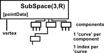 |
Points There is only one point and each point component has only one 'curve' and the 'curve' has only one point. |
 |
Curves Each curve component has only one curve and the curve has many indexes. |
 |
Polygons Each curve component has one curve with the first index and a second curve with the remaining indexes. |
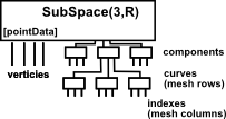 |
Meshes Each mesh component a curve for each row and each of these curves contains indexes for the columns. |
Documentation from code:
SubSpace(n:PI,R:Ring) : Exports == Implementation where n is the dimension of the subSpace The SubSpace domain is implemented as a tree. The root of the tree is the only node in which the field dataList - which points to a list of points over the ring, R - is defined. The children of the root are the top level components of the SubSpace (in 2D, these would be separate curves; in 3D, these would be separate surfaces). The pt field is only defined in the leaves. By way of example, consider a three dimensional subspace with two components - a three by three grid and a sphere. The internal representation of this subspace is a tree with a depth of three. The root holds a list of all the points used in the subspace (so, if the grid and the sphere share points, the shared points would not be represented redundantly but would be referenced by index). The root, in this case, has two children - the first points to the grid component and the second to the sphere component. The grid child has four children of its own - a 3x3 grid has 4 endpoints - and each of these point to a list of four points. To see it another way, the grid (child of the root) holds a list of line components which, when placed one above the next, forms a grid. Each of these line components is a list of points. Points could be explicitly added to subspaces at any level. A path could be given as an argument to the addPoint() function. It is a list of NonNegativeIntegers and refers, in order, to the n-th child of the -- current node. For example, addPoint(s,[2,3],p) would add the point p to the subspace s by going to the second child of the root and then the third child of that node. If the path does extend to the full depth of the tree, nodes are automatically added so that the tree is of constant depth down any path. By not specifying the full path, new components could be added - e.g. for s from SubSpace(3,Float) addPoint(s,[],p) would create a new child to the root (a new component in N-space) and extend a path to a leaf of depth 3 that points to the data held in p. The subspace s would now have a new component which has one child which, in turn, has one child (the leaf). The new component is then a point. |
SubSpaceComponentProperty
newpoint.spad
These components can have the following boolean properties:
- closed - (true or false) the last point is connected back to the first.
- solid - (true or false) each polygon is filled in.
SubSpaceComponentProperty applies to components of ThreeSpace and SubSpace structures.
ThreeDimensionalViewport
view3D.spad
ThreeDimensionalViewport defines the rendering of the graphical information into a two dimensional image, such as:
- Direction of viewing (camera position and direction)
- Magnification (camera zoom)
- Perspective
- Lighting
- Clipping of image
- Displaying axes
- Displaying Title
- Translations
- Colour Information
- Writing (exporting) to a file.
GraphImage
view2D.spad
Holds a two dimensional graph as a list of list of points with related information as follows:
Rep := Record(key: I, rangesField: RANGESF, unitsField: UNITSF, _
llPoints: L L P, pointColors: L PAL, lineColors: L PAL, pointSizes: L PI, _
optionsField: L DROP)
Basic Operations: makeGraphImage, pointLists, key, ranges, units, component, appendPoint, point, coerce, putColorInfo, figureUnits.
TwoDimensionalViewport
view2D.spad
Basic Operations: getPickedPoints, viewport2D, makeViewport2D, options, graphState, graphs, title, putGraph, getGraph, axes, units, points, region, connect, controlPanel, close, dimensions, scale, translate, show, move, update, resize ,write, reset, key.
ViewDefaultsPackage
viewDef.spad
ViewportDefaultsPackage describes default and user definable values for graphics
Basic Operations: pointColorDefault, lineColorDefault, axesColorDefault, unitsColorDefault, pointSizeDefault, viewPosDefault, viewSizeDefault, viewDefaults, viewWriteDefault, viewWriteAvailable, var1StepsDefault, var2StepsDefault, tubePointsDefault, tubeRadiusDefault
DrawOption
drawopt.spad
A list of DrawOption values can be passed to drawing routines such as 'makeViewport3D' which controls how the x-window is drawn. For example, most of the above examples are drawn with the 'toScale(true)' option.
Basic Operations: adaptive, clip, title, style, toScale, coordinates, pointColor, curveColor, colorFunction, tubeRadius, range, ranges, var1Steps, var2Steps, tubePoints, unit
todo: more explanation of the individual options.
see also (DrawOptionFunctions1(S:Type), DrawOptionFunctions0())
DrawComplex
drawpak.spad
provides some facilities for drawing complex functions
drawComplex(f:C -> C,rRange:S,iRange:S,arrows?:Boolean) -> ThreeDimensionalViewport
draws a complex function as a height field. It uses the complex norm as the height and the complex argument as the color. It will optionally draw arrows on the surface indicating the direction
of the complex value.
Sample call:
f z == exp(1/z)
drawComplexVectorField: (f:C -> C,rRange:S,iRange:S) -> ThreeDimensionalViewport
Draws a complex vector field using arrows on the x--y plane. These vector fields should be viewed from the top by pressing the "XY" translate button on the 3-d viewport control panel.
Sample call:
f z == sin z
drawComplexVectorField(f, -2..2, -2..2) -> ThreeDimensionalViewport
Call the functions setRealSteps to change the number of steps used in each direction.
TwoDimensionalPlotClipping
clip.spad
Automatic clipping for 2-dimensional plots. The purpose of this package is to provide reasonable plots of functions with singularities.
Various clip functions are provided to map Plot into:
Record(brans: L L Pt,xValues: SEG SF,yValues: SEG SF)
RealSolvePackage
acplot.spad
This package provides numerical solutions of systems of polynomial equations for use in ACPLOT.
- solve: (Polynomial Fraction Integer,Float) -> L Float
- solve(p,eps) finds the real zeroes of a univariate rational polynomial p with precision eps.
- solve: (Polynomial I,Float) -> L Float
- solve(p,eps) finds the real zeroes of a univariate integer polynomial p with precision eps.
- realSolve: (L Polynomial I,L Symbol,Float) -> L L Float
- realSolve(lp,lv,eps) = compute the list of the real solutions of the list lp of polynomials with integer coefficients with respect to the variables in lv, with precision eps.
PlaneAlgebraicCurvePlot
acplot.spad
Exports ==> PlottablePlaneCurveCategory with
makeSketch:(P I,SE,SE,SEG RN,SEG RN) -> %
makeSketch(p,x,y,a..b,c..d) creates an ACPLOT of the curve \spad{p = 0} in the region
a <= x <= b, c <= y <= d.
More specifically, 'makeSketch' plots a non-singular algebraic curve p = 0 in an rectangular region xMin <= x <= xMax,
Min <= y <= yMax.
The user inputs makeSketch(p,x,y,xMin..xMax,yMin..yMax).
Here p is a polynomial in the variables x and y with integer coefficients (p belongs to the domain Polynomial Integer). The case where p is a polynomial in only one of the variables is allowed. The variables x and y are input to specify the the coordinate axes. The horizontal axis is the x-axis and
the vertical axis is the y-axis. The rational numbers xMin,...,yMax specify the boundaries of the region in which the curve is to be plotted.
CoordinateSystems
coordsys.spad
CoordinateSystems provides coordinate transformation functions for plotting. Functions in this package return conversion functions which take points expressed in other coordinate systems and return points with the corresponding Cartesian coordinates.
Basic Operations: cartesian, polar, cylindrical, spherical, parabolic, elliptic, parabolicCylindrical, paraboloidal, ellipticCylindrical, prolateSpheroidal, oblateSpheroidal, bipolar, bipolarCylindrical, toroidal, conical
DenavitHartenbergMatrix
dhmatrix.spad
Homogeneous Transformations, projective space
A Denavit-Hartenberg Matrix is a 4x4 Matrix of the form:
| nx | ox | ax | px |
| ny | oy | ay | py |
| nz | oz | az | pz |
| 0 | 0 | 0 | 1 |
Which is used to represent a 3 dimensional isometry, a transform which is a combination of rotation and translation.
TopLevelDrawFunctionsForCompiledFunctions
draw.spad
implements draw and makeObject
GraphicsDefaults
grdef.spad
TwoDimensionalPlotSettings sets global flags and constants for 2-dimensional plotting.
Various Open Inventor Structures
IVNodeCategory, RenderTools, IVSimpleInnerNode, IVSeparator, IVGroup, IVCoordinate3, IVQuadMesh, IVIndexedLineSet, IVUtilities
Open Inventor, originally IRIS Inventor, is a C++ object oriented retained mode 3D graphics API designed by SGI to provide a higher layer of programming for OpenGL
invnode.as
see discussion on this thread:
http://lists.gnu.org/archive/html/axiom-developer/2002-11/msg00151.html
MoebiusTransform
moebius.spad
Defined algebraically - like: (a*x + b)/(c*x + d) but there doesn't seem to be a standard way to transform shapes and so on (perhaps in a coordinate independent way?)
Point
newpoint.spad
Represents a point in space, most graphical primitives are constructed from point. Equivalent to a vector applied to the origin.
extends PointCategory:
PointCategory
PointCategory is the category of points in space which may be plotted via the graphics facilities. Functions are provided for defining points and handling elements of points.
Basic Operations: point, elt, setelt, copy, dimension, minIndex, maxIndex, convert
PointPackage
newpoint.spad
Functions where 3D points can be represented in carteasian, spherical or cylindrical coodinates.
xCoord : POINT -> R
yCoord : POINT -> R
zCoord : POINT -> R
xCoord(pt) returns the first element of the point, pt, although no assumptions are made as to the coordinate system being used. This function is defined for the convenience of the user dealing with a Cartesian coordinate system.
rCoord : POINT -> R
rCoord(pt) returns the first element of the point, pt, although no assumptions are made as to the coordinate system being used. This function is defined for the convenience of the user dealing with a spherical or a cylindrical coordinate system.
thetaCoord : POINT -> R
thetaCoord(pt) returns the second element of the point, pt, although no assumptions are made as to the coordinate system being used. This function is defined for the convenience of the user dealing with a spherical or a cylindrical coordinate system.
phiCoord : POINT -> R
phiCoord(pt) returns the third element of the point, pt, although no assumptions are made as to the coordinate system being used. This function is defined for the convenience of the user dealing with a spherical coordinate system.
color : POINT -> R
color(pt) returns the fourth element of the point, pt, although no assumptions are made with regards as to how the components of higher dimensional points are interpreted. This function is defined for the convenience of the user using specifically, color to express a fourth dimension.
hue : POINT -> R
hue(pt) returns the third element of the two dimensional point, pt, although no assumptions are made with regards as to how the components of higher dimensional points are interpreted. This function is defined for the convenience of the user using specifically, hue to express a third dimension.
shade : POINT -> R
shade(pt) returns the fourth element of the two dimensional point, pt, although no assumptions are made with regards as to how the components of higher dimensional points are interpreted. This function is defined for the convenience of the user using specifically, shade to express a fourth dimension.
PointFunctions2
newpoint.spad
implements map : ((R1->R2),Point(R1)) -> Point(R2)
ParametricPlaneCurve
paramete.spad
ParametricPlaneCurve is used for plotting parametric plane curves in the affine plane.
also see ParametricPlaneCurveFunctions2 which implements:
map: (CF1 -> CF2, ParametricPlaneCurve(CF1)) -> ParametricPlaneCurve(CF2)
stored as:
Rep := Record(xCoord:ComponentFunction,yCoord:ComponentFunction)
ParametricSpaceCurve
paramete.spad
ParametricSpaceCurve is used for plotting parametric space curves in affine 3-space.
stored as:
Rep := Record(xCoord:ComponentFunction,_
yCoord:ComponentFunction,_
zCoord:ComponentFunction)
ParametricSurface
paramete.spad
ParametricSurface is used for plotting parametric surfaces in affine 3-space.
stored as:
Rep := Record(xCoord:ComponentFunction,_
yCoord:ComponentFunction,_
zCoord:ComponentFunction)
PlottablePlaneCurveCategory
pcurve.spad
PlottablePlaneCurveCategory is the category of curves in the plane which may be plotted via the graphics facilities. Functions are provided for obtaining lists of lists of points, representing the branches of the curve, and for determining the ranges of the x-coordinates and y-coordinates of the points on the curve.
PlottableSpaceCurveCategory
pcurve.spad
PlottableSpaceCurveCategory is the category of curves in 3-space which may be plotted via the graphics facilities. Functions are provided for obtaining lists of lists of points, representing the branches of the curve, and for determining the ranges of the x-, y-, and z-coordinates of the points on the curve.
Plot3D
plot3d.spad
Plot3D supports parametric plots defined over a real number system. A real number system is a model for the real numbers and as such may be an approximation. For example, floating point numbers and infinite continued fractions are real number systems. The facilities at this point are limited to 3-dimensional parametric plots.
Basic Operations: pointPlot, plot, zoom, refine, tRange, tValues, minPoints3D, setMinPoints3D, maxPoints3D, setMaxPoints3D, screenResolution3D, setScreenResolution3D, adaptive3D?, setAdaptive3D, numFunEvals3D, debug3D
Plot
plot.spad
The Plot domain supports plotting of functions defined over a real number system. A real number system is a model for the real numbers and as such may be an approximation. For example floating point numbers and infinite continued fractions. The facilities at this point are limited to 2-dimensional plots or either a single function or a parametric function.
see also: PlotFunctions1
PlotTools
plottool.spad
This package exports plotting tools
calcRanges: L L Pt -> L SEG SF
TubePlot
tube.spad
Package for constructing tubes around 3-dimensional parametric curves. Domain of tubes around 3-dimensional parametric curves.
also: TubePlotTools, ExpressionTubePlot, NumericTubePlot
ViewportPackage
viewpack.spad
Basic Operations: graphCurves, drawCurves
ViewportPackage provides functions for creating GraphImages and TwoDimensionalViewports from lists of lists of points.