Data Type

Most programming have a set of built-in data types and then ways to combine them to produce more complex data types, for instance,

Primitive Data Types

• Integer
• Float (real)
• Boolean (Logic)
• Character

There may also be some variations on these such as double precision.

The type definitions on this page use a programming language called 'Charity' (http://pll.cpsc.ucalgary.ca/charity1/www/home.html) which takes its ideas from category theory.

Combining Primitive Data Types

We can combine the above built-in types to form compound types in the following ways:

Union

This is where only one of the types applies at a given time.

We might want a type like Shape which could either be a Circle which requires a single float to define it (say radius) or alternatively a Rectangle which requires two floats to define it (say height and width).

type: Shape = Circle float | Rectangle float float

Another possibly might be where we require a function to normally return a numeric value but in case of an error, such as divide by zero, we want it to return a string containing an error message.

A similar concept is enumeration (enum)

Compound (Tuple)

Alternatively the compound type can contain both the data types being combined simultaneously. This is a bit like a fixed length list but where each element in the list could be a different type.

This page looks at data types as mathematical expressions which we can manipulate in equations.

Recursive Types

We can define compound types recursively. There are two ways to do this:

• Inductive data types, such as list, where the recursion is on the input and the instance on the output of the definition.
• Coinductive data types, such as stream, where the recursion is on the output and the instance on the input of the definition.

Algebraic Data Types

Languages such as Haskell and Idris allow types to be defined by listing their possible values, these are the constructors for the type.

These constructors can also be recursive allowing us to define infinite types such as natural numbers and lists.

Types defined in this way allow us to prove things about the type at compile time, especially if the type is defined as a free initial algebra such as natural numbers defined in terms of zero and successor constructors. We can then define plus in a way that we can prove what would otherwise be axioms.

Certain types, such as natural numbers and lists, are fully specified by these constructors. These are known as w-types [ref 1] . However more complex data types such as groups or graphs would be hard or impossible to fully define in this way although we can still construct something with the required functionality. For example, imagine we want to model a finite group and to do this we want to construct permutations. We could represent a permutation as a list of natural numbers where the value of the n-th item in the list represents the index of the entry it maps to. To be a valid permutation the list should contain every index once only but this is not enforced by the constructor.

data perm Nat
	    p : list Nat | p * (inv p) = 1

This sort of thing can be done in proof assistants but I don't know any general purpose languages with this ability.

Examples of Data Types

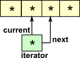	List Data Type This is inductive: Construction is simpler but readout (destruction) is more complicated.
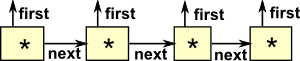	Stream Data Type This is coinductive: Construction is more complicated but readout (destruction) is simpler.

Combinatory Logic

For more information about combinatory logic see this page.

Object Oriented

In an object oriented program recursion can be used as follows:

Java - List

In java we encapsulate in an object

class List<E>
{
  E value;
  List<E> next;
}

Scala - Tree

case classes in scala are a halfway between encapsulating in an object and algebraic data types in functional languages.

abstract class Tree
  case class Sum(l: Tree, r: Tree) extends Tree
  case class Var(n: String) extends Tree
  case class Const(v: Int) extends Tree

The case class is similar to | in that it uses pattern matching.

Charity

terminology

where:

• x = W -> X
• y = W -> Y
• v = X -> W
• w = Y -> W

functor/mapping/function examples:

utilities:

data list A -> C = nil : 1     -> C
                 | cons: A * C -> C.

data SF A -> C = ss: A -> C
               | ff: 1 -> C.

data coprod(A, B) -> C = b0: A -> C
                       | b1: B -> C.

data bool -> C = false | true: 1 -> C.

data nat -> C = zero: 1 -> C
              | succ: C -> C.

Inductive Datatypes

data bTree (A, B) -> C = leaf: A           -> C
                       | node: B * (C * C) -> C.

Coinductive Datatypes

data T -> triple(A, B, C) = p0_3: T -> A
                          | p1_3: T -> B
                          | p2_3: T -> C.

data C -> conat = denat: C -> SF(C).

data C -> colist(A) = delist: C -> SF(A * C).

data C -> cobTree(A, B) = debTree: C -> A + (B * (C * C)).

Infinite Datatypes

data C -> infnat = poke: C -> C.

data I -> inflist(A) = head: I -> A
                     | tail: I -> I.

data C -> infbTree(B) = infnode: C -> B * (C * C).

Lazy Datatypes

data Eid A -> C = eid: A -> C.     % eager identify datatype
data C -> Lid A = lid: C -> A.     % lazy identify datatype

data C -> Lprod(A, B) = fst: C -> A
                      | snd: C -> B.

data Lnat -> N = Lzero: 1      -> N
               | Lsucc: Lid(N) -> N.

data Llist(A) -> L = Lnil : 1          -> L
                   | Lcons: A * Lid(L) -> L.

Higher-Order Datatype

The exponetial datatype: the datatype of total functions
data C -> exp(A, B) = fn: C -> A => B.

* the datatype of total, deteministic processes
data C -> proc(A, B) = pr: C -> A => B * C.
* the datatype of partial processes
data C -> Pproc(A, B) = Ppr: C -> A => SF(B * C).
* the datatype of nondeteministic processes
data C -> NDproc(A, B) = NDpr: C -> A => list(B * C).

data S -> stack(A) = push: S -> SF(A) => S
                   | pop : S -> S * SF(A).

data Q -> queue(A) = enq: Q -> SF(A) => Q
                   | deq: Q -> Q * SF(A).

EuclideanSpace

home

Prerequisites

The mathematics of type theory is discussed on this page.

This page discusses how complicated data types can be made up from primitive types. In object oriented languages this is done by creating new objects but, in other languages there are more direct methods of creating compound types, including inductive and coinductive data types.

Related Information

This page looks at data types as mathematical expressions which we can manipulate in equations.

The mathematics of this is discussed on this page: Type Theory

Functional Programming and Category Theory