The Scenegraph Concept
A scenegraph consists of a number of nodes in a tree structure, the types of nodes are:
- Root Node
- Group Node
- Line Node
- Indexed Face Set (IFS) Node
- Text Node
- Clip Node
- Material Node
- Transform Node
- Arrow Node
- Named Points Node
- Shape Node
- Def Node
- Use Node
This tree is constructed by starting with the root node and adding child nodes using the addChild! function as follows:
addChild!:(n:%,c:%) -> Void
where 'c' is the child node and 'n' node that it is being added to. Any node type can be a child node or a parent (although it only makes sense to put the root node only at the root).
In general a given node will affect only those nodes under it in the tree structure.
The purpose and constructors of these nodes is as follows: (in the following definitions PT refers to an instance of SPointCategory such as SCartesian,SArgand or SConformal).
Root Node
| Every scenegraph must have one root node and all other nodes must be added, in a tree structure, under this node (either directly or indirectly). So the root node can represent the whole scenegraph and it is what is passed to export routines, for example, to export the whole scenegraph. | 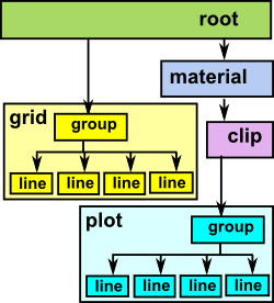 |
createSceneRoot:() -> %
createSceneRoot:(bb: SBoundary(PT)) -> %
createSceneRoot:(minx:I,miny:I,maxx:I,maxy:I) -> %
The parameters define the boundary. This bounding box is intended to be the area or volume in which the graphical objects are drawn, elements of the geometry outside this area will not necessarily be clipped (to be sure use a clipping node with the same boundary). The bounding box in the root node has these additional effects:
- When exported to a drawing or editing application this defines the default area available for display of the graphics on the screen.
- It allows some elements such as line widths, font sizes, width of arrow heads and so on to be scaled so that they are of an appropriate size for the overall screen area. In mathematical terms a line has no width but when drawing it we need to give it a nominal width so that it can be seen.
If the first version (without boundary information) is used then the boundary will be calculated, to include all the nodes, when the scene is first drawn to a file.
For more information about boundaries see page here.
Group Node
Constructs a group node, this node does not do anything itself but contains other nodes. Any node can contain other nodes - we do not need to use a group node to do this, but if we just want to group nodes without any other effects then this is a good choice.createSceneGroup:() -> % addSceneGroup:(n:%) -> %
addSceneGroup is a convenience function which combines the constructor createSceneGroup with addChild! This allows a scene graph node to be constructed and added to the scenegraph in one operation. Most of the scenegraph constructors have this form as an option.
Line Node
Constructs a line node, this contains a (possibly curved) line,represented by a list of points) in n-dimensional space. The dimension of the space is implicit in the type of points being used.
A Line node can hold a single line or multiple lines. The reason that a Line node needs to hold multiple lines is that, when a clip is applied to a line this might break it into several line segments.
The following form constructs a single line:
createSceneLine:(line: List PT) -> %
addSceneLine:(n:%,line: List PT) -> %
The following form constructs multiple lines:
createSceneLines:(line: LINES) -> %
addSceneLines:(n:%,line: LINES) -> %
Where: LINES==> List List PT
The following form constructs a single line where the endpoints are specified by nodes, the line is drawn upto the boundary of the nodes. This way of constructing lines is useful for drawing an 'edge' in graph theory.
- st is the node at the start of the line
- en is the node at the end of the line
createSceneLine:(st:%,en:%) -> %
addSceneLine:(n:%,st:%,en:%) -> %
Arrow Node
Constructs a arrow node, this contains a line or lines with an arrow head at the end in n-dimensional space. The dimension of the space is implicit in the type of points being used.
The size of the arrow head is controlled by 'mode' and 'size' parameters. 'mode' can have the following values:
- "fixed"::Symbol -- fixed size line width given by 'size' parameter
- "proportional"::Symbol -- size as a proportion of the overall bounds
- "variable"::Symbol -- size as a proportion of the arrow length
So "proportional" would typically be used when drawing a graph (in graph theory) where it looks better if each arrow head is the same. "variable" would typically be used when drawing a force field where a bigger arrow head might indicate a stronger force.
createSceneArrows:(line: List List PT,mode:Symbol,size:DF) -> %
addSceneArrows:(n:%,line: List List PT,mode:Symbol,size:DF) -> %
The following form constructs an arrow where the endpoints are specified by names from named points node:
createSceneArrow:(st:String,en:String,offset:PT,mode:Symbol,size:DF) -> %
addSceneArrow:(n:%,st:String,en:String,offset:PT,mode:Symbol,size:DF) -> %
The following form constructs a single arrow where the endpoints are specified by nodes, the arrow is drawn upto the boundary of the nodes. This way of constructing arrows is useful for drawing an directed edge in graph theory.
- st is the node at the start of the arrow
- en is the node at the end of the arrow
createSceneArrow:(st:%,en:%,offset:PT,mode:Symbol,size:DF) -> %
addSceneArrow:(n:%,st:%,en:%,offset:PT,mode:Symbol,size:DF) -> %
More about arrows here.
Indexed Face Set (IFS) Node
Constructs an indexed face set node, this defines a surface in n-dimensional space represented by a set of polygons in n-dimensional space.
createSceneIFS:(inx: List List NNI,pts: List PT) -> %
    addSceneIFS:(n:%,inx: List List NNI,pts: List PT) -> %
    createSceneIFS:(in1: SceneIFS(PT)) -> %
    addSceneIFS:(n:%,in1: SceneIFS(PT)) -> %
A specialised constructor for an IFS node constructs a 3D box. Constructs an indexed face set node which is a 3D box of a given size
createSceneBox:(size:DF) -> %
    addSceneBox:(n:%,size:DF) -> %
Text Node
Constructs a text node, text can be used for labelling anything such as graphs, axes and so on.
createSceneText:(text: TEXT) -> %
    addSceneText:(n:%,text: TEXT) -> %
    createSceneText:(str:String,sz:NNI,pz:PT) -> %
    addSceneText:(n:%,str:String,sz:NNI,pz:PT) -> %
where: TEXT==> Record(txt:String,siz:NNI,pos:PT) which defines the text to be printed with its size and position.
Clip Node
Constructs a clip node, clips its sub nodes in the coordinate system in force at the clip node.
createSceneClip:(bb: SBoundary(PT)) -> %
addSceneClip:(n:%,bb: SBoundary(PT)) -> %
where: bb is the boundary that the node is clipped to.
Material Node
Constructs a material node
This sets:
- lineWidth,
- lineCol
- fillCol
- opacity
for all nodes under it, unless overridden by another material node. That is the material parameters that apply to a given node are those of the closest material node above it in the hierarchy
createSceneMaterial:(mat:MATERIAL) -> %
addSceneMaterial:(n:%,mat:MATERIAL) -> %
createSceneMaterial:(lineW:DF,lineC:String,fillC:String) -> %
addSceneMaterial:(n:%,lineW:DF,lineC:String,fillC:String) -> %
Where: MATERIAL==> Record(lineWidth:DF,lineCol:String,fillCol:String)
Transform Node
Constructs a transform node
This transforms the points and vectors below this node If a given node has more than one transform node above it in the hierarchy then the transforms are concatenated (combined).
createSceneTransform:(tran:TR) -> %
addSceneTransform:(n:%,tran:TR) -> %
Or once the transform has already been created we can change the transform it represents, without altering the scene heirachy, this may be useful to create animations for example:
setTransform!:(n:%,tran:TR) -> Void
where tran is of type STransform(PT) and may be constructed in one of the following ways:
Construct with given matrix elements:
stransform: (m:List List DF) -> %
Construct transform in general form as a mapping from PT to PT:
stransform: (gen:PT -> PT) -> %
Construct transform as function of complex variable can only be used when PT is SArgand so this can be converted to PT -> PT:
stransform: (cpx:C -> C) -> %
Construct with a multivector:
stransform: (m: List DF) -> %
Construct transform which represents pure translation ++ we can also combine with scale which, for instance, is useful when writing to SVG file because the y dimension is inverted:
stranslate: (offsetx:DF,offsety:DF,offsetz:DF,scalex:DF,_
                 scaley:DF,scalez:DF) -> %
returns the identity element which is do nothing transform:
identity: () -> %
For more information about transformations see page here.
Shape Node
A shape is something like a rectangle or an ellipse in 2 dimensions or a sphere or box in 3 dimensions.
Its main purpose here, especially in 2 dimensions, is to provide a way to graphically show sets or visually associate things together. That is, the shape could be drawn around other elements to show that they are a set. For example we could draw Venn diagrams or show how one set of elements maps to another set of elements.
Of course we could create a shape by plotting the equation for that shape, for example, by using 'ParametricPlaneCurve'. However that would be unnecessarily complicated when we just want a shape to visually show a grouping of elements, the mathematical properties of the shape are not the issue here.
The shape is stored as follows:
SHAPE ==> Record(shptype:Symbol,centre:PT,size:PT,fill:Boolean) |
where:
- 'shptype' may have the following values:
- "rect"::Symbol
- "ellipse"::Symbol
- "box"::Symbol
- "sphere"::Symbol
- centre determines where the shape is drawn.
- size determines the extent of the shape (which may be different in each dimension).
- fill, if set to true, will fill the shape with the current fill colour. otherwise, if set to false, the inside of the shape is transparent.
  addSceneLines:(n:%,line: LINES) -> %
    ++ a convenience function which combines createSceneLines with addChild!
  createSceneShape:(shape:SHAPE) -> %
    ++ This just creates the shape without adding it.
|
A tutorial showing examples of how to use the shape node is here.
Named Points Node
The aim of the 'named points' node and associated domain is to provide better support for drawing graphs (that is 'graphs' as in graph theory) and diagrams of trees, latices and category theory arrow diagrams. In other words, diagrams with named nodes and arrows or lines between these nodes.
createSceneNamedPoints:(np:SceneNamedPoints PT) -> %
    ++ createSceneNamedPoints(np) constructs a named points node, this
    ++ allows us to define a set of points which can be used multiple
    ++ times in the scenegraph.
addSceneNamedPoints:(n:%,np:SceneNamedPoints PT) -> %
    ++ addSceneNamedPoints(n,np) is a convenience function which
++ combines createSceneNamedPoints with addChild! |
A tutorial showing examples of how to use the named point node is here.
Def Node
The 'def' and 'use' constructs are used together to allow us to include a branch of the scenegraph multiple times in the scene.
createSceneDef:(nam:String,nde:%) -> %
    ++ createSceneDef(nam,nde) defines a point in the scenegraph
    ++ so that it can be used elsewhere.
addSceneDef:(n:%,nam:String,nde:%) -> %
    ++ addSceneDef(n,nam,nde) is a convenience function which
++ combines createSceneDef with addChild! |
A tutorial showing examples of how to use the def and use nodes is here.
Use Node
The 'def' and 'use' constructs are used together to allow us to include a branch of the scenegraph multiple times in the scene.
createSceneUse:(nam:String) -> %
    ++ createSceneUse(nam) uses another point in the scenegraph.
addSceneUse:(n:%,nam:String) -> %
    ++ addSceneUse(n,nam) is a convenience function which
    ++ combines createSceneUse with addChild!
|
A tutorial showing examples of how to use the def and use nodes is here.
Drawing Plots and grids
The following constructors create 'compound' nodes in that the node returned has subnodes under it.
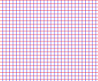
Grids and Patterns
Grids are useful as a background to plots, they consist of various straight, horizontal and vertical lines.
Since the lines in grids are defined by the endpoints of the lines, it does not make sense to apply a non-linear transform to them as the lines will remain straight and won't be transformed as they should.
Patterns are used to show the effect of transforms. Although they may be approximated by straight lines the points are intended to be close enough together to transform reasonably accurately.
Grid - The form with step uses the prevailing colour and thickness and the stepSize parameter defines the spacing between lines in local coordinates. createSceneGrid:(stepSize:DF_
,bb: SBoundary(PT)) -> %
addSceneGrid:(n:%,stepSize:DF,_
bb: SBoundary(PT)) -> % |
 |
Grid - The form without the step size constructs a grid with:
createSceneGrid:(bb: SBoundary(PT)) -> % addSceneGrid:(n:%,bb: SBoundary(PT)) -> % |
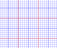 |
Pattern GRID - horizontal and vertical lines Contruct a set of horizontal and vertical lines in the current clip boundary and current material with a spacing between lines given by the step parameter. createScenePattern:_
("GRID"::Symbol,_
step:NNI,bb: SBoundary(PT)) -> %
addScenePattern:_
(n:%,"GRID"::Symbol,_
step:NNI,bb: SBoundary(PT)) -> % |
 |
Pattern SIERPINSKI- Sierpinski fractel Constructs a Sierpinski fractel. step parameter gives the level of subdivision. createScenePattern:_
("SIERPINSKI"::Symbol,_
level:NNI,bb: SBoundary(PT)) -> %
addScenePattern:_
(n:%,"SIERPINSKI"::Symbol,_
level:NNI,bb: SBoundary(PT)) -> % |
 |
Pattern 3 - HOUSE createScenePattern:_
("HOUSE"::Symbol,_
level:NNI,bb: SBoundary(PT)) -> %
addScenePattern:_
(n:%,"HOUSE"::Symbol,_
level:NNI,bb: SBoundary(PT)) -> % |
|
Ruler Creates a scale that can be used to provide numeric values for an axis:
createSceneRuler:_
  (ptype:Symbol,_
          offset:PT,bb: SBoundary(PT)) -> %
addSceneRuler:_
   (n:%,ptype:Symbol,_
offset:PT,bb: SBoundary(PT)) -> % |
One Dimensional subspace in Two Dimensions
This represents 1 dimension (line - possibly curved) in 2 dimensions (plane) The line is approximated as end-to-end straight lines defined by a list of points. In theory a line has no width but in that case we would not see it so we give it a width given by the material node that is applicable in this part of the scene graph.
The plot is defined by a function and a range of values. There are various ways to define this function:
- DF -> DF a mapping from float to float
- DF -> PT a mapping from float to point
Where:
DF ==> DoubleFloat
PT ==> SPointCategory -- an instance of SPointCategory represents a point.
We can also create the plot using an indirect parameter. (parametric)
PPC is ParametricPlaneCurve(DF -> DF) which is created with curve(f1,f2)
where f1 and f2 are functions of type ComponentFunction, in this case DF -> DF
createPlot1Din2D: (f:DF -> PT,tRange:SEG,numPts:NNI) -> %
addPlot1Din2D: (n:%,f:DF -> PT,tRange:SEG,numPts:NNI) -> %
createPlot1Din2D: (DF -> DF,SEG,numPts:NNI) -> %
addPlot1Din2D: (n:%,DF -> DF,SEG,numPts:NNI) -> %
createPlot1Din2Dparametric: (PPC,SEG,numPts:NNI) -> %
addPlot1Din2Dparametric: (n:%,PPC,SEG,numPts:NNI) -> %
One Dimensional subspace in Three Dimensions
create a line (1D subspace) in 3D space. This represents 1 dimension (line - possibly curved) in 3 dimensions. In theory a line has no width but in that case we would not see it so we give it a width given by the material node that is applicable in this part of the scene graph.
Again there are various ways to define this function:
PCFUN is a function from float to point: DF -> PT
PSC ParametricSpaceCurve(DF -> DF) is created with curve(f1,f2,f3)
where f1,f2 and f3 are functions of type ComponentFunction, in this case DF -> DF
createPlot1Din3Dparametric: (PSC,SEG,numPts:NNI) -> %
addPlot1Din3Dparametric: (n:%,PSC,SEG,numPts:NNI) -> %
createPlot1Din3Dparametric: (PCFUN,SEG,numPts:NNI) -> %
addPlot1Din3Dparametric: (n:%,PCFUN,SEG,numPts:NNI) -> %
Two Dimensional subspace in Three Dimensions
create a surface (2D subspace) in 3D space
The surface is approximated by polygons which are represented by in indexed face set (IFS) node:
createPlot2Din3D: (ptFun:PSFUN,uSeg:SEG,vSeg:SEG,numPts:NNI) -> %
createPlot2Din3D: ((DF,DF) -> DF,SEG,SEG,numPts:NNI) -> %
addPlot2Din3D: (n:%,(DF,DF) -> DF,SEG,SEG,numPts:NNI) -> %
createPlot2Din3Dparametric: (PSFUN, SEG, SEG,numPts:NNI) -> %
addPlot2Din3Dparametric: (n:%,PSFUN, SEG, SEG,numPts:NNI) -> %
createPlot2Din3Dparametric: (PSF,SEG,SEG,numPts:NNI) -> %
addPlot2Din3Dparametric: (n:%,PSF,SEG,SEG,numPts:NNI) -> %
Arrows
Displays multiple arrows on the screen. This is represented by a list, each element in this list represents a single arrow, This is represented by a list containing the start and end points.
createSceneArrows:(line: List List PT,ls:NNI,le:NNI) -> %
addSceneArrows:(n:%,line: List List PT,ls:NNI,le:NNI) -> %
We can represent transforms using arrows in various ways. The following example displays the function 'fn' which maps each point to a point 50 units to its right.
DF ==> DoubleFloat
fn(x:SCartesian(2)):SCartesian(2) ==
   spnt(screenCoordX(x)$SCartesian(2) +50::DF,_
     screenCoordY(x)$SCartesian(2))$SCartesian(2)
view:= boxBoundary(sipnt(0,0)$SCartesian(2),_
            sipnt(1200,1000)$SCartesian(2))
sc := createSceneRoot(view)$Scene(SCartesian(2))
gd := addArrows2Din2D(sc,fn,_
       1..1000,1..1000,15)$Scene(SCartesian(2))
writeSvg(sc,"exampleArrow2.svg") |
|

Exporting the graphics
This scenegraph framework currently exports to the following file formats:
- SVG - For 2 dimensional graphics this is the most standards based and also supported by graphical editors such as Inkscape.
- X3D - For 3 dimensional graphics I think this is the most standards compliant but it is not supported on many 3D editors.
- VRML - VRML2 and VRML97 are supported but not VRML1. This flavour of VRML holds the same information as X3D but using a different non-XML syntax.
- Wavefront(obj) - This is a very simple 3D format that will hold meshes but not text or colour information. It is supported on most 3D editors but only use it as a fallback if the other 3D formats don't work.
To export a scenegraph to one of these file formats use the following function calls:
Write an 'SVG' representation of node 'n' (usually the root node) to the filename supplied:
writeSvg:(n:%,filename:String) -> Void
Or we can do the same, but this version outputs all points using integer values, since the drawing width is usually normalised to be a 1000 units across this should give enough resolution and will make the file a lot smaller:
writeSvgQuantised:(n:%,filename:String) -> Void
Write an 'X3D' representation of node 'n' (usually the root node) to the filename supplied.
writeX3d:(n:%,filename:String) -> Void
Write a 'VRML' representation of node 'n' (usually the root node) to the filename supplied.
writeVRML:(n:%,filename:String) -> Void
Write an 'OBJ' (Wavefront) representation of node 'n' (usually the root node) to the filename supplied.
writeObj:(n:%,filename:String) -> Void
If we only want to create an XML structure without writing to a file we can use these functions:
create an XmlElement containing a 'SVG' representation of node 'n' and the nodes below it:
toSVG:(n:%,mat:MATERIAL,tran:TR,bb: SBoundary(PT)) -> XmlElement
Create an XmlElement containing a 'X3D' representation of node 'n' and the nodes below it:
toX3D:(n:%,mat:MATERIAL,tran:TR,bb: SBoundary(PT)) -> XmlElement
Creates .OBJ (Wavefront) structures from scenegraph tree structure called recursively for each node, so when called on root node in scenegraph all other nodes in the scenegraph will get called. When called the reference values should be empty or zero and when the function returns they will be set.
toObj:(n:%,ptLst: Reference List PT,_
    indexLst:Reference List List NNI,_
    indexNxt:Reference NNI,tran:TR,bb: SBoundary(PT)) -> Void
Compiling the code
This code is availible in FriCAS since FriCAS 1.1.1 but if you need to install a later version see page here.
Further Information
- User Tutorial on this page.
- Tutorial2 - conformal space.
- Programmers Reference on this page.
- Examples of scenegraph structure on this page.
- The code is in file: scene.spad.pamphlet which is available from here.
- Existing Axiom graphics framework on this page.